Aggregate Supply
Aggregate Supply. Tells us how much is produced in goods and services in the country. Determinant of Aggregate Supply. Prices Wages and Prices of Other Inputs (raw materials) Capital stock State of Technology Expectations. Aggregate Supply.

Aggregate Supply
E N D
Presentation Transcript
Aggregate Supply Tells us how much is produced in goods and services in the country.
Determinant of Aggregate Supply • Prices • Wages and Prices of Other Inputs (raw materials) • Capital stock • State of Technology • Expectations
Aggregate Supply Holding: Wages, Prices of Other Inputs Capital stock State of Technology and Expectations constant Holding all other determinants of supply constant Relationship between the price level and the Quantity of Real GDP supplied
Aggregate Supply Shows the relationship between Prices and Output Supplied
Important Difference: • Price: what the producer sells output for. The price is paid by the ultimate user • Cost: what the producer pays for raw materials, labor and other expenses necessary to produce. When costs rise, each unit is more expensive to produce, the producer must raise price to cover the increase in cost. The change in costs occurs first The change in price occurs as a result of the increase in cost.
Wages are rigid, “sticky” in the short run • Labor union contracts, wages change only when the contract expires. • Minimum wage laws • Workers do not accept lower wages easily. • Firms are reluctant to cut wages afraid to lose most productive workers and negatively affect productivity and morale. • Firms and workers know the recession will not last and thus “wait out” the bad times refusing to budge.
How do firms decide how much to produce? • Firms maximize profits • Profit per unit = Price per unit – Cost per unit. • Labor costs (wages and salaries) are “sticky” in the short run. • If labor is the ONLY cost of production then • When Prices increase, given that wages (costs) remain constant, profits increase: the firm reacts by producing moreunits • When Prices decrease, given that wages (costs) remain constant, profits decrease : the firm reacts by producing fewer units If prices rise while wages and other costs are fixed, production becomes more profitable and firms produce more. The Aggregate Supply Curve slopes upward in the short run: higher pricesresult in higher production
Aggregate Supply Curves Slopes Upward Short Run Aggregate Supply= SRAS Price Level Real GDP supplied
Movement Along Aggregate Supply • When Prices increase, given that wages (costs) remain constant, profits increase and the firm will react by producing more units • When Prices decrease, given that wages (costs) remain constant, profits decrease and the firm will react by producing fewer units Changes in Prices cause a movement along Aggregate Supply
Shiftsin the Aggregate Supply Curve • Prices • Wages and prices of Other Inputs • Capital stock: labor and Physical capital • Technology/Productivity AS shifts to the left as firms produce less when their costs increase. AS shifts to the right as firms produce more with a larger labor force or a larger stock of physical capital. AS shifts to the right as firms produce more with better technology.
Determining the Price Level The price level is the result of the interplay between Aggregate Demand and Aggregate Supply. To determine the price level, we must put Aggregate Demand and Aggregate Supply together.
120 100 80 Y Y AE AE Y=AE Determining the Price Level Price index Excess Supply: AE < Y, inventories rise, firms decrease both production and prices Aggregate Supply AS EQUILIBRIUM: AE = Y, inventories unchanged, firms do not change production or prices Aggregate Demand AD Excess Demand: AE > Y, inventories drop, firms increase both production and prices. 6,400 5,600 6,000 0 Real GDP
If G, I, a, NX increase AE line Shifts up Equilibrium Income increases Aggregate demand increases 45 Price level AE1= C+I+G+NX AE0= C+I+G+NX Aggregate Expenditures P0 AD1 AD0 Y0 Y1 Y0 Y1 Real GDP Real GDP
The Aggregate Supply Curve Potential GDP Only Prices rise At Full Employment Closer to Full Employment Prices Increase Prices do Not change Below full employment Output Increases Output can not increase Output Increases
Smallest effect Largest effect For which segment does an increase in demand has the smallest/largest effect on output?
The Self Adjusting Mechanism How is it supposed to work?
Adjusting to an Inflationary Gap Economy’s self correcting mechanism to close an inflationary gap Prices rise, inflationary gap closes: purchasing power of wealth decreases, AD decreases ( a movement up along AD) AS2 Potential GDP AS1 Labor market shortages: Difficult for firms to hire, easy for workers to win wage increases P1 Inflationary Gap 100 Price level Wages rise: AS shifts left as labor costs rise AD0 5,000 4,000 Real GDP
If wages and prices do not fall: self correcting mechanism operates only weakly to cure recessions Adjusting to a Recessionary Gap Unemployment: easy for firms to hire, difficult for workers to win wage increases Potential GDP AS1 Prices fall, gap closes: purchasing power increases, AD increases AS2 Price level 100 Recessionary Gap P1 AD0 Wages fall: AS shifts right as labor costs decrease 5,000 6,000 Real GDP
The effect of an Increase in Demand 1. Economy starts at Potential GDP 2. Inflationary gap appears 3. Prices rise, output drops back to Potential GDP Economy ends at Potential GDP SRAS2 AS2 Potential GDP = LRAS Potential GDP AS1 In the Short Run AS has a positive slope In the Long Run AS is Vertical at Potential GDP 3 AS shifts left as labor costs rise P2 Inflationary Gap 2 AD increases P1 In the long run (ignoring the temporary move to point 2) the economy always ends up at potential GDP P0 Price level 1 AD1 AD0 5,000 4,000 Real GDP
Does the US economy has a self correcting mechanism? YES • When the economy experiences an inflationary gap, wages increase, shifting the AS left, increasing prices and thus slowing down AD. • When the economy experiences a recessionary gap, wages decrease, shifting the AS right, decreasing prices and thus increasing AD. BUT • This mechanism works slowly so there is an argument to be made in favor of stabilization policies.
Using the Model Stagflation from a Supply Shock: Rising Energy Prices shift the AS left
Stagflation from a Supply Shock AS2 AS1 Higher prices & lower output: stagflation P1 100 Oil Prices rise: AS shifts left Price level AD0 5,000 Real GDP
Determinants of consumption • Changes in wealth • shift the consumption function. • Example: value of stocks, bonds, consumer durables. • Changes in consumer expectations • Shift the consumption function. • Example: Pessimistic expectations decrease autonomous consumption. • Prices • Affect the purchasing power of assets. Shift up in AE line Shift right in AD line Shift up in AE line Movement Along AD line
Determinants of Investment • Interest Rates: • Tax Incentives: • Technical Change: • Expectations about the strength of demand: • Political Stability and the rule of law: Shift AE line Shift AD line
Government expenditures are determined by the budget process: The president, Congress and the Senate. Government expenditures Shift AE line Shift AD line Fiscal Policy
Determinants of Net Exports • National Incomes • GDP of other countries • Relative Prices • Exchange Rates Shift AE line Shift AD line
Shifts in the Aggregate Supply Curve • Prices • Wages and prices of Other Inputs • Capital stock: labor and Physical capital • Technology/Productivity AS shifts to the left as firms produce less when their costs increase. AS shifts to the right as firms produce more with a larger labor force or a larger stock of physical capital. AS shifts to the right as firms produce more with better technology.
Which graph describes the effect of an increase in Autonomous Consumption Near Full employment Below Full Employment Near Full employment Below Full Employment
Increased oil prices • Increase in autonomous consumption • Adverse supply shock with increase in government spending • Rising wage rates • Increase in labor productivity B A D C E Which graph best describes the effect of the following events
2. Recession caused by a decrease in consumption and increase in productivity 3. Recession & deflation mainly caused by drop in AD 2 3 5 4.Expansion with inflation caused mainly by increase in AD Which graph best describes the effect of the following events • Economic growth and inflation 5.Expansion with deflation mainly caused by increase in AS 1 4 5
Questions to prepare for the Quiz Draw both an AE – 45degree line and an AS-AD diagram to show the effect on GDP and the price level resulting from the following events: • A Decrease in interest rates. • Oil prices drop (a drop in costs of production). • Pessimistic business forecasts lead businesses to reduce their planned investment.
Questions to prepare for the quiz • A tax cut on business. • Increase in government spending. • A major increase in home prices • U.S pulls troops out of Iraq. • Manufacturers rush to acquire the new technology for producing zero emissions cars. • Overall prices increase (CPI increases) • Europeans impose tariffs on imported goods • U.S. retaliates by imposing tariffs on European goods
If G, I, a, NX increase AE line Shifts up Equilibrium Income increases 45 Price level AE1= C+I+G+NX DY = DG (1/1-MPC) AE0= C+I+G+NX Aggregate Expenditures P0 AD1 DY = DG (1/1-MPC) AD0 Y0 Y1 Y0 Y1 Real GDP Real GDP
Inflation Reduces the Size of the Multiplier AD Shifts by the full multiplier amount DY = DG (1/1-MPC) If firms DO NOT raise prices AS1 Excess Demand: AE > Y, inventories drop, firms increase both production and prices. P1 P0 Price level AD1 If firms DO raise prices, the increase in output is SMALLER than given by the multiplier formula AD0 Y0 Y1 Y2 Real GDP
The Aggregate Supply Curve Only Prices rise At Full Employment Closer to Full Employment Prices Increase Prices do Not change Below full employment Output can not increase no multiplier effect Output Increases by less than multiplier Output Increases by full multiplier
Smallest multiplier effect Largest multiplier effect Which segment has the smallest/largest multiplier effect?
a. Decrease in interest rates d. a tax cut on purchase of equipment g. rush to acquire new technology: increases Investment, AE, Equilibrium Output, AD, Prices and GDP. AS0 AE1 P1 AE0 P0 AD1 AD0 Y0 GDP0 GDP1 Y1
c. Pessimistic forecast: Decreases Investment, AE, Equilibrium Output, AD, Prices and GDP. AS0 AE0 AE1 P0 P1 AD1 AD0 Y1 Y0 GDP1 GDP0
e. Increase in home prices: increases real value of wealth , consumption, AE, Equilibrium Output, AD, Prices and GDP. AS0 AE1 P1 AE0 P0 AD1 AD0 Y0 GDP0 GDP1 Y1
e.Overall Prices Decrease: increases wealth (in real terms), increase in Consumption, AE, Equilibrium Output, movement along AD AS0 AE1 AE0 P0 P1 AD1 AD0 Y0 GDP0 GDP1 Y1
f. U.S. pulls troops out of Iraq: Decreases Government Spending, AE, Equilibrium Output, AD, Prices and GDP. AS0 AE0 AE1 P0 P1 AD1 AD0 Y1 Y0 GDP1 GDP0
e. U.S. imposes tariffs on European goods: Decreases Imports, increases net exports, AE, Equilibrium Output, AD, Prices and GDP. AS0 AE1 P1 AE0 P0 AD1 AD0 Y0 GDP0 GDP1 Y1
i. Europeans impose tariffs on imported goods: Decreases Exports, AE, Equilibrium Output, AD, Prices and GDP. AS0 AE0 AE1 P0 P1 AD1 AD0 Y1 Y0 GDP1 GDP0
An adverse supply shock: oil prices increase, wages increase AS1 AS0 P1 P0 AD0 GDP1 GDP0
A favorable supply shock (drop in cost of production or increase in productivity): wages drop, oil prices drop AS0 AS1 P0 P1 AD0 GDP0 GDP1