Binary Trees
Binary Trees. CSC 220. Your Observations (so far data structures). Array Unordered Add, delete, search Ordered Linked List ??. Introduction to Tree. Fundamental data storage structures used in programming. Combines advantages of an ordered array and a linked list.

Binary Trees
E N D
Presentation Transcript
Binary Trees CSC 220
Your Observations (so far data structures) • Array • Unordered • Add, delete, search • Ordered • Linked List • ??
Introduction to Tree • Fundamental data storage structures used in programming. • Combines advantages of an ordered array and a linked list. • Searching as fast as in ordered array. • Insertion and deletion as fast as in linked list.
Tree (example) node edge Draw a parse tree
Tree characteristics • Consists of nodes connected by edges. • Nodes often represent entities (complex objects) such as people, car parts etc. • Edges between the nodes represent the way the nodes are related. • Its easy for a program to get from one node to another if there is a line connecting them. • The only way to get from node to node is to follow a path along the edges.
Tree Terminology • Path: Traversal from node to node along the edges results in a sequence called path. • Root: Node at the top of the tree. • Parent: Any node, except root has exactly one edge running upward to another node. The node above it is called parent. • Child: Any node may have one or more lines running downward to other nodes. Nodes below are children. • Leaf: A node that has no children. • Subtree: Any node can be considered to be the root of a subtree, which consists of its children and its children’s children and so on.
Tree Terminology • Visiting: A node is visited when program control arrives at the node, usually for processing. • Traversing: To traverse a tree means to visit all the nodes in some specified order. • Levels: The level of a particular node refers to how many generations the node is from the root. Root is assumed to be level 0. • Keys: Key value is used to search for the item or perform other operations on it.
Binary Trees • Every node in a binary tree can have at most two children. • The two children of each node are called the left child and right child corresponding to their positions. • A node can have only a left child or only a right child or it can have no children at all. • Left child is always less that its parent, while right child is greater than its parent.
Applet • ..\FinalApplets\Chap08\Tree\Tree.html
Unbalanced Trees • Some trees can be unbalanced. • They have most of their nodes on one side of the root or the other. Individual subtrees may also be unbalanced. • Trees become unbalanced because of the order in which the data items are inserted. • If the key values are inserted in ascending or descending order the tree will be unbalanced. • For search-centric application (Binary tree), an unbalanced tree must be re-balanced.
Is a binary tree ADT? • What are tree behaviors? • Do they look familiar to other DS? • Implantation details? • Draw UML diagram for a B-Tree?
Representing Tree in Java • Similar to Linked List but with 2 Links • Store the nodes at unrelated locations in memory and connect them using references in each node that point to its children. • Can also be represented as an array, with nodes in specific positions stored in corresponding positions in the array.
Btree Btree Btree Btree Int data Btree left_chid Btree right_child Int data Btree left_chid Btree right_child Int data Btree left_chid Btree right_child Int data Btree left_chid Btree right_child Find() Insert() Delete() Find() Insert() Delete() Find() Insert() Delete() Find() Insert() Delete() Object with links
Traversing the Tree • Visiting each node in a specified order. • Three simple ways to traverse a tree: • Inorder • Preorder • Postorder
Inorder Traversing Inorder traversal will cause all the nodes to be visited in ascending order. • Steps involved in Inorder traversal (recursion) are: • -- Call itself to traverse the node’s left subtree • -- Visit the node (e.g. display a key) • -- Call itself to traverse the node’s right subtree. inOrder( node lroot) { If (lroot != null) { inOrder(lroot.leftChild()); System.out.print(lroot.iData + “ “); inOrder(lroot.rightChild()); }
Tree Traversal (continued) • Sequence of preorder traversal: e.g. use for infix parse tree to generate prefix -- Visit the node -- Call itself to traverse the node’s left subtree -- Call itself to traverse the node’s right subtree • Sequence of postorder traversal: e.g. use for infix parse tree to generate postfix -- Call itself to traverse the node’s left subtree -- Call itself to traverse the node’s right subtree -- Visit the node.
Finding a Node • To find a node given its key value, start from the root. • If the key value is same as the node, then node is found. • If key is greater than node, search the right subtree, else search the left subtree. • Continue till the node is found or the entire tree is traversed. • Time required to find a node depends on how many levels down it is situated, i.e. O(log N).
Inserting a Node • To insert a node we must first find the place to insert it. • Follow the path from the root to the appropriate node, which will be the parent of the new node. • When this parent is found, the new node is connected as its left or right child, depending on whether the new node’s key is less or greater than that of the parent. • What is the complexity?
Finding Maximum and Minimum Values • For the minimum, • go to the left child of the root and keep going to the left child until you come to a leaf node. This node is the minimum. • For the maximum, • go to the right child of the root and keep going to the right child until you come to a leaf node. This node is the maximum.
Deleting a Node • Start by finding the node you want to delete. • Then there are three cases to consider: • The node to be deleted is a leaf • The node to be deleted has one child • The node to be deleted has two children
Deletion cases: Leaf Node • To delete a leaf node, simply change the appropriate child field in the node’s parent to point to null, instead of to the node. • The node still exists, but is no longer a part of the tree. • Because of Java’s garbage collection feature, the node need not be deleted explicitly.
Deletion: One Child • The node to be deleted in this case has only two connections: to its parent and to its only child. • Connect the child of the node to the node’s parent, thus cutting off the connection between the node and its child, and between the node and its parent.
Deletion: Two Children • To delete a node with two children, replace the node with its inorder successor. • For each node, the node with the next-highest key (to the deleted node) in the subtree is called its inorder successor. • To find the successor, • start with the original (deleted) node’s right child. • Then go to this node’s left child and then to its left child and so on, following down the path of left children. • The last left child in this path is the successor of the original node.
Efficiency • Assume number of nodes N and number of levels L. • N = 2L -1 • N+1 = 2L • L = log(N+1) • The time needed to carry out the common tree operations is proportional to the base 2 log of N • O(log N) time is required for these operations.
Huffman Code • Binary tree is used to compress data. • Data compression is used in many situations. E.g. sending data over internet. • Character Code: Each character in a normal uncompressed text file is represented in the computer by one byte or by two bytes. • For text, the most common approach is to reduce the number of bits that represent the most-used characters. • E.g. E is the most common letter, so few bits can be used to encode it. • No code can be the prefix of any other code. • No space characters in binary message, only 0s and 1s.
Creating Huffman Tree • Make a Node object for each character used in the message. • Each node has two data items: the character and that character’s frequency in the message. • Make a tree object for each of these nodes. • The node becomes the root of the tree. • Insert these trees in a priority queue. • They are ordered by frequency, with the smallest frequency having the highest priority. • Remove two trees from the priority queue, and make them into children of a new node. • The new node has frequency that is the sum of the children’s frequencies. • Insert this new three-node tree back into the priority queue. • Keep repeating these two steps, till only one tree is left in the queue.
Coding the Message • Create a code table listing the Huffman code alongside each character. • The index of each cell would be the numerical value of the character. • The contents of the cell would be the Huffman code for the corresponding character. • For each character in the original message, use its code as an index into the code table. • Then repeatedly append the Huffman code to the end of the coded message until its complete.
Creating Huffman Code • The process is like decoding a message. • Start at the root of the Huffman tree and follow every possible path to a leaf node. • As we go along the path, remember the sequence of left and right choices, regarding a 0 for a left edge and a 1 for a right edge. • When we arrive at the leaf node for a character, the sequence of 0s and 1s is the Huffman code for that character. • Put this code into the code table at the appropriate index number.