Download

1 / 17
180 likes | 378 Vues
Sea Surface Salinity from a global ocean mixed layer model. Sylvain Michel, Jean Tournadre, Bertrand Chapron and Nicolas Reul Laboratoire d'Océanographie Spatiale, IFREMER Brest, France. Plan. 1. Introduction 2. Coherent description of the ocean surface 3. Mixed layer model configuration

E N D
Sea Surface Salinity from a global ocean mixed layer model • Sylvain Michel, Jean Tournadre, Bertrand Chapron and Nicolas Reul • Laboratoire d'Océanographie Spatiale, IFREMER • Brest, France
Plan • 1. Introduction 2. Coherent description of the ocean surface 3. Mixed layer model configuration 4. Inversion of the mixed layer depth 5. Variability and global balance of SSS • 6. Conclusions
Ocean Observations Panel for Climate (OOPC):usefulness of surface salinity data in the context of climate change detection "At high latitude, sea surface salinity is known to be critical for decadal and longer time scale variations associated with deep ocean over-turning and the hydrological cycle. In the tropics, and in particular in the western Pacific, Indonesian Seas, and in upwelling zones, salinity is also believed to be important." • -> benchmark sampling strategy: • one sample per 200 km square, • every 10 days, • with an accuracy of 0.1 psu SSS data distribution (blue: n=1, red: n>10) in the World Ocean Atlas 2001 in situ climatology (NODC)
1. Introduction: SSS remote sensing based on microwave emissivity at band L (1.4 Ghz) • Soil Moisture and Ocean Salinity (ESA) • - 69 radiometers (interferometry) • - multiple incidence angles, H&V polarisations • - launch in early 2007 (duration>3 years) • - nominal resolution: 50 km, 3 days -> accuracy=1.0 psu • - after averaging : 200 km, 10 days -> accuracy=0.1 psu • Aquarius/SAC-D (NASA/CONAE) • - 1 radiometer + 1 scatterometer • - launch in March 2009 (duration=3 years) • - 150 km, 1 month -> accuracy=0.2 psu
1. Introduction : objectives • Technical: prepare SMOS mission • - calibration/validation • - first guess for the inversion algorithm • qualification of the inversed salinity and the associated fluxes Scientific : study SSS variability - physical processes governing its evolution - important environmental parameters - understanding of measurement errors Geophysical mechanisms influencing SSS remote sensing,from Aquarius/SAC-D website (NASA) -> work at the interface of remote sensing and physical oceanography
2. Coherent description of the ocean surface:2D « slab mixed layer » model horizontal current (from satellite data) : Ekman transport + geostrophic current vertical entrainment (if we > 0) :Ekman pumping + diapycnal mixing entrainment : if we > 0, =1 / if we < 0, =0
3. Mixed layer model configuration: simulation design ERA40 reanalysis: 1948-2001 / SSALTO-DUACS analysis : August 2001-2005 -> use of daily climatological forcing fields Implementation : - global domain (80°S-80°N), ECMWF grid, resolution: x = y = 1.125° - daily climatological forcing - monthly Td et Sd vertical profiles - constant horizontal diffusivity: = 2000 m2.s-2 - time-step t = 1 day / 1 hour (depends on the integration mode) wind stress (in N/m2), annual mean, ERA40 reanalysis geostrophic current (in m/s), annual mean, SSALTO-DUACS analysis
Qnet E-P-R Tmod Tpro(t)=T(t-1)+T h(t)=MLD Tobs Tdia(t)=SST(t-1)+T Ugeo SST Smod Spro(t)=S(t-1)+S Td(z) Sd(z) Sdia(t)=Sd(t-1)+S 3. Mixed layer model configuration: 2 integration modes • diagnostic mode (constrained SST/SSS) -> heat and salt balances • prognostic mode (free SST/SSS) -> temperature and salinity evolution
4. Mixed layer depth: result of the inversion from SST • values: different from in situ estimates • global distribution: good qualitative agreement - winter convection regions - minimum over Tropics - deepening in strong current areas Mixed layer depth (in m) in March, from the daily climatological simulation (top) and from the thermocline T(10m)-0.2°C of the climatology by De Boyer-Montégut et al., 2003 (bottom)
4. Mixed layer depth: validation of the inversion • time correlation C: • C > 0.8 over most of the global ocean • -> observed and simulated MLDs evolve in phase • C 0 • - inconsistency between current, fluxes and/or SST (shelves, western boundaries) • - strong sensitivity to errors in air-sea fluxes (ITCZs) • C < 0 • - ignored processes (sea ice, mesoscale circulation) • - lack of in situ measurements • -> restrict geographically the study of SSS from the simulation time correlation between - the inverted MLD from the daily climatological simulation (monthly means) - the T02 thermocline depth from De Boyer-Montégut et al. (2003)
5. Variability and balance of SSS: annual mean distribution simulated SSS distribution comparable to observations. ex.: maxima in subtropical gyres, minima in tropical bands high shifts reveal problems : - inadequate model (ex.: polar seas) - erroneous fluxes (ex.: ITCZs) - fluxes/currents inconsistency (ex.: AACC) Sea Surface Salinity (in psu), annual mean, from the daily climatological simulation (top)and from the World Ocean Atlas 2001 climatology (bottom)
6. Global salinity balance: standard deviations of the 6 processes (in 10-3 psu/day) geostrophic advection Ekman advection diapycnal mixing Ekman pumping freshwater flux lateral diffusion
5. Global salinity balance: dominant processes Global contributions (in % of the ice-free ocean surface): geostrophic advection 33% air-sea flux 22% diapycnal mixing 22% Ekman advection 13% lateral diffusion 8% Ekman pumping 3% • dominant process for the SSS variations at each model point, from the daily climatological simulation
6. Conclusions • Technical objectives: • -method for SSS estimate from remote sensing data • - qualification of the fluxes associated with the SSS inversion • -> developed tool: 2D « slab mixed layer » model • - ensures the consistency between parameters measured by various sensors (synthesis of satellite observations) • - enables to close the surface balances (kinetic momentum, heat and salt) • - easy to implement and fast to compute (operational applications) • - 2 integration modes (analysis and forecast) • Mixed Layer Depth: • - critical parameter in the model • - only variable non accessible from satellite observations • - original inversion method providing a MLD estimate adapted to the model, compatible with the observations • -> geographical restrictions (model simplicity, fluxes/currents/SST inconsistency) • -> elsewhere, inverted MLD = link between forcing and ocean properties
7. Conclusions Scientific objectives: • SSS variability - global distribution: higher time/space resolution than in situ climatology - estimate high-frequency variability (1 day < t < 1 month) - comparison with observations: good overall agreement - determine the mechanisms responsible for the SSS variability • Salinity balance • more complex than in the case of temperature: • role of atmospheric flux: less predominant -> lower impact of E-P flux uncertainties • - diapycnal mixing important in some areas • -> estimates of T, S vertical profiles • - increased importance of advection, principally geostrophic • -> interest for high-resolution currents inferred from altimetry
7. Perspectives • Perspectives: • use of a satellite-only forcing (QuikSCAT, LOS, SAFO-SI, SSALTO-DUACS, GPCP) • interannual simulation (1990-2005) • increased resolution (1° -> 1/4°) • improvement in the equatorial band (use of a complex friction for Ekman current) • high latitudes: include the freshwater flux due to sea-ice • Applications: • - SMOS calibration/validation (1st guess, independent SSS estimate) • - freshwater flux adjustment from SSS- air-sea fluxes consistency with observations of surface properties (SST, SLA, color) • - study of the SSS impact on deep water formation (thermohaline circulation) • - study of the SSS impact SSS on water masses ventilation (CO2 trapping)