Mixed Layer
Mixed Layer. P. N. Vinayachandran Centre for Atmospheric and Oceanic Sciences (CAOS) Indian Institute of Science (IISc) Bangalore 560 012. Summer School on Dynamics of North Indian Ocean June-July 2010. Outline. Mixed Layer Air-sea fluxes Models of Mixed Layer Bulk Models

Mixed Layer
E N D
Presentation Transcript
Mixed Layer P. N. Vinayachandran Centre for Atmospheric and Oceanic Sciences (CAOS) Indian Institute of Science (IISc) Bangalore 560 012 Summer School on Dynamics of North Indian Ocean June-July 2010
Outline Mixed Layer Air-sea fluxes Models of Mixed Layer Bulk Models Kraus – Turner Price, Weller & Pinkle (PWP) Profile Models K-Profile Parameterizaion Meller Yamada
Mixed Layer Near – surface layer of the ocean. Quasi homogeneous Properties (T, S, ) are nearly uniform in this layer The layer where properties change rapidly with depth is thermocline Importance: Weather and climate (eg. cyclones) Air – sea exchange is controlled my mixed layer processes Life in the ocean: Most of the primary productivity occurs in the mixed layer i) Most of the electromagnteic radiation is absorbed within the mixed layer Ii) Mixing at the base of the mixed layer is crucial for sustaining biological productivity
How do we determine the depth of the mxed layer Vinayachandran et al., 2002, JGR
Difference Criterion Properties are assumed to be uniform within the mixed layer Isothermal, Isohaline and Isopycnal Temperature: 0.1 to 1.0C ( 0.2 C ) Density: 0.01 to 0.25 kg m-3 (0.03 km m-3) Gradient Criterion Properties are assumed to change `sharply' just below the mixed layer
Air – sea fluxes Radiation Shortwave Downwelling radiation Day of the year Zenith angle Latitude Atmospheric transmittance (aerosol and water vapour) Cloud cover Upwelling shortwave radiation Reflection from the sea surface Albedo, Clear sky radiation, fractional cloud cover, noon solar elevation
Net Shortwave Radiation SOC Flux data set. Josey, 1999
Penetration of short wave radiation Solar radiation in the uppper ocean is given by I(z) = I(0 )∑ nez/Ln I(0) = insolation at the surface N = no. of spectral bands Ln = length scale i) shortwave (UV < 350nm) e-folding scale of UV ~ 5m ii) visible (PAR 350 – 700nm) part that penetrates Iii) IR and nIR (> 700nm) absorbed in the top 10cm I(z) = I(0) [I1 ez/L1 - I2 ez/L2] L1 = 0.6 L2 = 20m I1 = 0.62 I2 = 1 - I1 Paulson and Simpson, 1977, JPO
Longwave Radiation Incoming: Radiation from the atmosphere Outgoing: Radiation from the sea surface Longwave Downwelling longwave radiation Air temperature and humidity Upwelling longwave radiation Reflection of longwave radiation Emission from the sea surface a Emittance of the sea surface Vapor pressure Cloud cover coefficient (0.5 to 0.73)
Sensible heat flux QH = ra Cp w'T' QH = ra Cp Ch u (Ts - Ta)
Latent heat flux QE = ra L w 'q' QE = ra L Ce u (qs - qa)
Net heat flux QN = QSW + QLW + QE + QH
Surface Buoyancy Flux B = ro [ a (roCp) -1 Qnet – b So (E – P) ] ro = surface density So = surface salinity a, b = Expansion coefficients for heat and salt Cp= heat capacity Positive buoyancy flux is stabilizing
Source: Oberhuber (siign reversed)
Mixed layer processes Heating by solar radiation: Penetrative Cooling by evaporation, mechanical mixing Heating/Cooling : Sensible heat flux/Longwave radiation There is no echange of salt Freshwater exchange by Evaporation and Precipitation Changes buoyancy flux
Kraus – Turner Bulk Mixed Layer Model Kraus & Turner, Tellus, 1967a: Experimental Kraus & Turner, Tellus, 1967b: Theory
Schemtic of the mixed layer Denman, 1973, JPO
Assumptions • Incompressible ocean. • Stably stratified fluid (Boussinesq approximation) • Wave-like dynamical effects ignored (Gravitational, inertial and Rossby waves) • Horizontal homogenity, neglect horizontal advection Turbulent heat flux at the base of the mixed layer
Entrainment Integrate from z= -h to z=-h+△h 0 at z=-h In the limit as △h 0 ≤ 0 ; no entrainment; H=0 ≥ 0 ; entrainment mixing ; H=1
Calculation of Entrainment Velocity Production of TKE m is an adjustable parameter; B is the buoyancy flux 1. If P > 0 ; entrainment deepening of mixed layer 2. If P < 0 ; relative importance of winds v/s convection Monin-Obukhov Length McCreary et al., 2001
Wind dominated regime Wind speed = 12.5 m/s; No heat flux, No radiation h after 24 hours = 37.1; after 48 hours = 47.8 Denman, JPO, 1973
Wind dominated regime Run 1. Wind speed = 12.5 m/s Run 2. Wind speed = 17 m/s
Diurnal Heating Wind speed = 4 m/s; Profiles are plotted evey 2hrs
The PWP (Price Weller Pinkel) Model Price et al., 1986, JGR
The (PWP) ice Weller Pinkel Model F(0)=Q, air-sea heat flux E(0)=S(E-P), fresh water flux times surface salinity G(0)= , wind stress
Kelvin-Helmholtz Instability Wikepedia Instability due to vertical shear in a stratifed fluid
Mixing Static stability Mixed layer stability Shear flow stability h mixed layer depth difference between mixed layer and the level just beneath. Rb bulk richardson number Rg gradient richardson number
Implementation • Vertical grid resolution, ∆z =0.5 m ; Time step, ∆t = 900 s • Begin from an initial T, S profile (eqns. 1 & 2) • Update the T, S profile for the first grid box, all the surface heat flux goes in here • Update T profile for the boxes 2 to N using penetrative part of radiaion • Calculate density using an equation of state, calculate mixed layer depth for a density criterion of 0.0001 • Check for static stabiity, mix and remove all instability • Calculate veloctiy profile using winds (eqn. 3) • Check for mixed layer stability, Rb > 0.65, mix and remove instability • Check for shear flow instability, Rg > 0.25, mix and remove instability
Rg assumed to be ≥ 0.25 If the smallest Rg < 0.25 , then , T, S and V at the two grid levels that produce Rg , j and j+1 are partially mixed according to, is the value after mixing ; Rg' = 0.3 Rg is then recalculated from (j-1) to (j+2) and the mixing process continues until Rg ≥ 0.25.
KPP Mixed Layer The turbulent mixing in the oceanic boundary layer is distinctly different from the layer below Vertical extent of oceanic boundary layer depends on surface forcing, stratificcation and shear Depth upto which an eddy in the boundary layer can penetrate before becoming stable. Shallowest depth where Rb > 0.3 Monin-Obukhov Length: Large and Gent, 1999, JPO
Below the boundary layer (interior) vertical mixing consists of: 1. Local Ri due to instability due to resolved vertical shear 2. internal wave breaking 3. double diffusion