Chapter 5 NEURAL NETWORKS
Chapter 5 NEURAL NETWORKS. by S. Betul Ceran. Outline. Introduction Feed-forward Network Functions Network Training Error Backpropagation Regularization. Introduction. Multi-Layer Perceptron (1).

Chapter 5 NEURAL NETWORKS
E N D
Presentation Transcript
Chapter 5NEURAL NETWORKS by S. Betul Ceran
Outline • Introduction • Feed-forward Network Functions • Network Training • Error Backpropagation • Regularization
Multi-Layer Perceptron (1) • Layered perceptron networks can realize any logical function, however there is no simple way to estimate the parameters/generalize the (single layer) Perceptron convergence procedure • Multi-layer perceptron (MLP) networks are a class of models that are formed from layered sigmoidal nodes, which can be used for regression or classification purposes. • They are commonly trained using gradient descent on a mean squared error performance function, using a technique known as error back propagation in order to calculate the gradients. • Widely applied to many prediction and classification problems over the past 15 years.
Multi-Layer Perceptron (2) • XOR (exclusive OR) problem • 0+0=0 • 1+1=2=0 mod 2 • 1+0=1 • 0+1=1 • Perceptron does not work here! Single layer generates a linear decision boundary
Universal Approximation 1st layer 2nd layer 3rd layer Universal Approximation: Three-layer network can in principle approximate any function with any accuracy!
Feed-forward Network Functions (1) • f: nonlinear activation function • Extensions to previous linear models by hidden units: • Make basis function Φ depend on the parameters • Adjust these parameters during training • Construct linear combinations of the input variables x1, …, xD. (2) • Transform each of them using a nonlinear activation function (3)
Cont’d • Linearly combine them to give output unit activations (4) • Key difference with perceptron is the continuous sigmoidal nonlinearities in the hidden units i.e. neural network function is differentiable w.r.t network parameters • Whereas perceptron uses step-functions Weight-space symmetry • Network function is unchanged by certain permutations and the sign flips in the weight space. • E.g. tanh(– a) = –tanh(a) ………flip the sign of all weights out of that hidden unit
Two-layer neural network zj: hidden unit
A multi-layer perceptron fitting into different functions f(x)=x2 f(x)=sin(x) f(x)=H(x) f(x)=|x|
Network Training • Problem of assigning ‘credit’ or ‘blame’ to individual elements involved in forming overall response of a learning system (hidden units) • In neural networks, problem relates to deciding which weights should be altered, by how much and in which direction. • Analogous to deciding how much a weight in the early layer contributes to the output and thus the error • We therefore want to find out how weight wij affects the error ie we want:
Two schemes of training • There are two schemes of updating weights • Batch: Update weights after all patterns have been presented(epoch). • Online: Update weights after each pattern is presented. • Although the batch update scheme implements the true gradient descent,the second scheme is often preferred since • it requires less storage, • it has more noise, hence is less likely to get stuck in a local minima (whichis a problem with nonlinear activation functions). In the online updatescheme, order of presentation matters!
Problems of back-propagation • It is extremely slow, if it does converge. • It may get stuck in a local minima. • It is sensitive to initial conditions. • It may start oscillating.
Regularization (1) • How to adjust the number of hidden units to get the best performance while avoiding over-fitting • Add a penalty term to the error function • The simplest regularizer is the weight decay:
Changing number of hidden units Over-fitting Sinusoidal data set
Regularization (2) • One approach is to choose the specific solution having the smallest validation set error Error vs. Number of hidden units
Consistent Gaussian Priors • One disadvantage of weight decay is its inconsistency with certain scaling properties of network mappings • A linear transformation in the input would be reflected to the weights such that the overall mapping unchanged
Cont’d • A similar transformation can be achieved in the output by changing the 2nd layer weights accordingly • Then a regularizer of the following form would be invariant under the linear transformations: • W1: set of weights in 1st layer • W2: set of weights in 2nd layer
Early Stopping • A method to • obtain good generalization performance and • control the effective complexity of the network • Instead of iteratively reducing the error until a minimum of the training data set has been reached • Stop at the point of smallest error w.r.t. the validation data set
Effect of early stopping Training Set Error vs. Number of iterations Validation Set A slight increase in the validation set error
Invariances • Alternative approaches for encouraging an adaptive model to exhibit the required invariances • E.g. position within the image, size
Various approaches • Augment the training set using transformed replicas according to the desired invariances • Add a regularization term to the error function; tangent propagation • Extract the invariant features in the pre-processing for later use. • Build the invariance properteis into the network structure; convolutional networks
Tangent Propagation(Simard et al., 1992) • A continuous transformation on a particular input vextor xn can be approximated by the tangent vector τn • A regularization function can be derived by differentiating the output function y w.r.t. the transformation parameter, ξ
Tangent vector implementation Tangent vector corresponding to a clockwise rotation Original image x True image rotated Adding a small contribution from the tangent vector x+ετ
References • Neurocomputing course slides by Erol Sahin. METU, Turkey. • Backpropagation of a Multi-Layer Perceptron by Alexander Samborskiy. University of Missouri, Columbia. • Neural Networks - A Systematic Introduction by Raul Rojas. Springer. • Introduction to Machine Learning by Ethem Alpaydin. MIT Press. • Neural Networks course slides by Andrew Philippides. University of Sussex, UK.