Download
1 / 34
360 likes | 632 Vues
Land Use Theory and Models. Man Li, Research Fellow International Food Policy Research Institute Technical Training for Modeling Scenarios for Low Emission Development Strategies, September 9 th –20 th , 2013. Outline. The Von Thünen model Introduction

E N D
Land Use Theory and Models Man Li, Research Fellow International Food Policy Research Institute Technical Training for Modeling Scenarios for Low Emission Development Strategies, September 9th–20th, 2013
Outline • The Von Thünenmodel • Introduction • Modeling land use with micro-level data • Modeling land use when data are mixed at micro- and aggregate level
The Von Thünen Model • Economists generally turn to a class of models pioneered in the early 19th century by Johann Heinrich von Thünen when dealing with the questions of how economy organizes its use of space
The Von Thünen Model • Von Thünen developed the basics of the theory of land rent in a mathematically rigorous way R = Y(p-c)-YFD R = land rent Y = yield per unit of land p = market price per unit of commodity c = production expenses per unit of commodity F = freight rate (per commodity unit per mile) D = distance to market
Von Thünen’s Assumptions • The city is located centrally within an "Isolated State" which is self-sufficient and has no external influences • The Isolated State is surrounded by wilderness • The land is completely flat and has no rivers or mountains
Von Thünen’s Assumptions • Soil quality and climate are consistent • There are no roads. Farmers in the Isolated State transport their own goods to market across land directly to the central city. • Farmers behave rationally to maximize profits
Von Thünen’s Rings • Vegetables/fruit/milk must get to market quickly • Wood was important for heating and cooking but difficult to transport • Grains last longer than dairy products and are much lighter than wood • Animals can be raised far from city since they are self-transporting The black dot represents a city; 1 (white) dairy and intensive farming; 2 (green) timber and firewood; 3 (yellow) extensive field crops like grain; 4 (red) ranching; the outer, dark green area represents wilderness where agriculture is not profitable
Weaknesses and Criticism • The model did not take into account differences in sites, can be modified by relaxing some conditions: • Differential transportation costs, e.g., boats • Variations in topography • Soil fertility • Changes in demand or price of the commodity • Nevertheless, the model tends to hold true in most instances
Land Use Data • To a large extent, the scope and method of empirical studies are driven by the data available • Aggregate vs. disaggregate • Continuous vs. Discrete
Aggregate Data • County, province, or national data • E.g., Lichtenberg 1989 AJAE; Stavins and Jaffe 1990 AER; Wu and Segerson 1995 AJAE; Hardie and Parks 1997 AJAE; Miller and Plantinga 1999 AJAE • Assuming a SINGLE “representative” agent makes land use decisions • Acreage response model is often specified as a linear model, a logit functional form, a probit functional form, etc.
Some Limitations of Aggregate Data • Aggregation problem • Under what conditions can the distribution of individual characteristics be ignored • A large body of literature suggests these conditions are quite STRICT and “aggregate bias” does exist in many empirical studies • Prediction accuracy (aggregate vs. disaggregate) • Less attention in the literature • Results vary with different applications • CANNOT be resolved by a priori reasoning even in the context of linear prediction models (Wu and Adams 2002 JARE)
Micro-level Data(or Disaggregate Data) • Survey data • E.g., Lubowski et al. 2006 JEEM; Lewis and Plantinga 2007 Land Econ • Remote-sensing land cover data • E.g., Chomitz and Gray 1996 WBER; Nelson and Hellerstein 1997 AJAE; Pfaff 1999 JEEM; Deininger and Minten 2002 AJAE; etc.
Micro-level Data • Conceptual basis: micro-parameter distribution model or random utility model • Can partly control heterogeneous site-characteristics over space, such as soil type, terrain slope, access to market, etc. (many studies) • Can take into account spatial externalities • i.e., spatial interactions b/w neighboring agents (Irwin and Bockstael 2002 JEG) or b/w nearby land parcels (Li et al. 2013 Land Econ)
Some Limitations of Micro-level Data • Spatial econometric concerns • Difficulty in identification • Spatial heterogeneity or spatial dependence • Spatial error dependence or spatial lag dependence • Spatial error dependence (unobserved factors that are correlated over space • In linear model: invalid hypothesis testing procedure • In nonlinear models: biased estimates • Spatial lag dependence (spatial interactions) • Still limited application because of estimation challenge • Intensive computation • Sampling routine
When Land Use are Discrete Choices • Recall von Thünen’s Model: R = Y(p-c)-YFD • Let i be land plot, j be land use choice • In a reduced form: Rij = pijY(pij,wij)-wijX(pij,wij) • Following von Thünen, assume pij=p(i) andwij=w(Di)
When Land Use are Discrete Choices • Rewrite land rent as Rij = Ziβj + εij • Assume land is devoted to the highest-rent use: plot i is devoted to use j if Rij > Rik, for all k ≠ j (1) • Under some assumptions of ε, (1) is equivalent to a multinomial logit model in which Prob(i devoted to j) = . (2)
When Land Use are Continuous Shares • Consider a farmer i, s/he owns land area Ai in total and has J options to allocate land. • Her/his problem becomes to choose aij≥0 to maximize the restricted total profits s.t. . • With some mathematical arrangement, . (3)
When Land Use are Continuous Shares • Eq.(3) can be estimated using a flexible functional form, such as translog or normalized quadratic, for the restricted profit function then derive the implied functional form for the share equations • Advantage: providing a theoretical link b/w profit function and share equations • Disadvantage • Desirable local properties do not necessary hold globally • Does not ensure predicted shares lie in the 0-1 interval
When Land Use are Continuous Shares • Alternatively, can assume a functional form for the share equations themselves, e.g., logistic form • Ensures predicted shares lie b/w 0 and 1 • The logistic model has been shown to outperform other flexible functional forms and has been widely applied in economic analysis
Some More Complicated Problems • Land use change refers to more than simply the pattern of different land covers (e.g., cropland, grassland, rangeland) in space • Rather, it includes any changes in arrangements, activities, and inputs that people undertake in a certain land cover type • Those activities, however, are rarely available with a finer spatial resolution (e.g., parcel-level or pixel-level)
Exercise • Divide into 3–4 groups • Discuss the factors affecting land use/land use change in your country • Find common factors among countries, and factors distinguished from other countries • Present and compare b/w groups and countries
Group Discussions • Common factors (Vietnam & Bangladesh): • Climate change • Sea-level rise: affect agricultural soil quality and induce soil salinity • Land degradation • Distinguished factors: • Vietnam: • Food security policy can be ensured because the government controls land use • Commune makes land use planning (especially for coffee and tea) • Annual crops are likely to be driven by markets • Bangladesh: • Fragmental land parcel owned/managed by several farmers • Shrimp farming leads to soil salinity • Subsidy/tax are important incentive policies affecting land allocation • Administrative hierarchy: National/Division/District/Sub-district/Union (Agro-ecological zone) • Government makes recommendations on fertilizer application, cropping calendar, etc. through internet • Colombia: • No government plan, farmers can make land use decisions themselves • Distance to river and geophysical characteristics are important factors affecting farmers’ decision • Market driven
Section IV: Modeling land use when data are mixed at micro- and aggregate level ―A Spatial Nested Land Use Model
Land Use Model Structure: Two-level Nested Logit Decision Maker Cropland Mosaic of Cropland Shrub/ Grassland Forests Other Uses Upper Level Beans Cassava Cotton Groundnuts Maize Rice Soybean Sugarcane Sweet potatoes … Lower Level
Model Specification: Upper Level • Choice variable: Land cover (MODIS or GLC2000) • Note this variable is usually available with fine resolution, e.g., 500 meters or 1 km
Model Specification: Upper Level • Explanatory variables • Socioeconomic factors: population density, market access • Site-specific variables: elevation, terrain slope, soil PH • Climate variables: annual precipitation, annual mean temperature • Institutional factors: protected area (dummy variable) • Variable as a link to the lower-level model: estimated inclusive values from the lower-level model
Model Specification: Lower Level • Choice variable: Provincial-/county-level share of harvested area for each crop • Note unlike the choice variable at the upper-level, this variable are NOT available with fine resolution • Explanatory variables • Crop suitability • Crop price (spatially explicit, one period lag) • Inertia variable (lagged crop area)
Estimation Procedure • Estimate the nested model in a sequential fashion from the lower level to the upper level • Maximum likelihood method • Analysis unit • Lower level: Province/county • Upper level: land grid
A government plan to pave roads in the DRC • The government plans to pave 8,500 km of roads and improve railways, ferries and boats (Ulimwengu et al. 2009) Planned Road Expansion (Simulation) Current Road Network (Baseline)
The percentage increase in agricultural land per 1×1 km pixel