Simulation
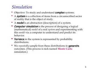
Simulation. Based on Law & Kelton, Simulation Modeling & Analysis, McGraw-Hill. Why Simulation?. Test design when cannot analyze System too complex Can analyze only for certain cases (Poisson arrivals, very large N, etc.) Verify analysis Fast production of results. Simulation types.


Simulation
E N D
Presentation Transcript
Simulation Based on Law & Kelton, Simulation Modeling & Analysis, McGraw-Hill
Why Simulation? • Test design when cannot analyze • System too complex • Can analyze only for certain cases (Poisson arrivals, very large N, etc.) • Verify analysis • Fast production of results
Simulation types • Static vs. dynamic • Deterministic vs. stochastic • Continuous vs. discrete • Simulation model system model
Discrete Event System • Discrete system • The system state can change only in a countable number of points in time! • Event = an instantaneous change in state. • Example: a queueing system • System state: Number of customer • At each time number of customer can only change by an integer
Continuous Simulation • Simulating the flight of a rocket in the air • System state: rocket position and weight • State changes continuously in time (according to a partial differential equation)
Components of a discrete-event simulation model • System state: the collection of state variables necessary to describe the system at a particular time. • Simulation clock: a variable giving the current value of simulated time • Event list: a list containing the next time when each type of event will occur. • Statistical counters: variables used for storing statistical information about system performance • How many moments?
Components of a discrete-event simulation model (2) • Initialization routine: a subprogram to initialize the simulation model at time 0. • Timing routine: a subprogram that determines the next event from the event list and then advances the simulation clock to the time when the event is to occur. • Event routine: A subprogram that updates the system state when a particular type of event occurs (one routine per event).
Components of a discrete-event simulation model (3) • Library routine: A set of subprograms used to generate random observations from probability distributions that were determined as part of the simulation model. • Report generator: A subprogram that computes estimates (from the statistical counter) of the desired performance measures when simulation ends.
Components of a discrete-event simulation model (4) • Main program: a subprogram that invokes the timing routine to determine the next event and then transfers control to the corresponding event routine to update the system state. May also check for termination and invoke the report generator.
Flow control Init Determine next event Event 1 Event n Done? no report
Examplea single server queuing system • System to be simulated • Ai Interarrival times are I.I.D. • Si Service time are I.I.D. • FIFO service • Work preserving • Initial state • Empty and idle • First arrival after Ai time units from time 0 • Termination after n customers left queue.
Performance measures • d(n)=expected average delay in queue. • Customer point of view • q(n) = expected time-average number of customers in queue. • System point of view • Note: average over time which is continuous!! • u(n) = proportion of time server is busy
No. of customers in queue. Q(t) 4 3 2 1 0 t
No. of customers in queue. Q(t) 4 3 2 1 0 t
Performance measures (2) • Averages are not always enough. • Register max/min values. • Register the entire “pdf” • histograms
Initialization • Set simulation time to 0. • Set initial state: • Server idle • Queue empty • Last event time • Init event list • Generate 1st arrival • Zero stat counters • Total delay and number delayed • Area under Q(t) and B(t).
1st Event: customer arrival • After init finished the arrival event is selected and time is advanced to this event • Change server from idle to busy • Add 0 to total delay, increment No of delayed. • Generate two events: • This customer departure • Next arrival (generate as you go) • Add 0 to the area under Q(t). • Add 0 to the area under B(t).
2nd Event: customer arrival • Arrival event is selected and time is advanced to this event • Server busy => put customer in queue with arrival time • Set “No. in queue” to 1. • Generate next-arrival events (don’t mess with dep.) • Add 0 to the area under Q(t). • Add (t2-t1) to the area under B(t).
Remarks • While handling an event time is standing • But, order of operation is still important: • First update area under Q(t) then update “No. in queue” • Two events at the same time • Order may change simulation result!
Determining Events • In complex systems events sequence may not be trivial. • Use of event graph to aid us in designing the events
Event Graph • States are bulbs, connected with arrows • Bold arrow: event may occur. • Thin arrow: event must occur. depar- ture arrival
Alternative Event Graph • This design is correct as well! • One more event => more complexity • Simplification rule: • If an event node has incoming arcs that are all thin and smooth, it can be eliminated. • A strongly connected connected component that have no incoming arcs from other nodes must be initialized. Enter service depar- ture arrival
Take care • GIGO = garbage in garbage out • Realistic scenarios (arrival process, service time) • Full cover of system behavior • Statistical confidence • What to model • Not enough details => hurts accuracy • Too many details => slows simulation • Attempt to verify correctness • Simulate cases you can analyze
Random Generator • Make sure you can regenerate your random sequence, or debugging is hell. • For long simulations, use 32 bit pseudo random generator. 16 bit is too short!
Statistical Confidence • Better a few short runs than one long run. • However, make sure run time is long enough to make end conditions negligible. • option: start statistics after a while. • Given a set of IID random variables we can calculate the confidence interval.
Confidence Interval • X1, X2, …Xn are IID random variable with finite mean and finite variance 2>0. Fn(z)=P(Znz) is Dist. Func. of Zn • By central limit theorem Fn(z)(z) (the std. Normal r.v.) • For sufficiently large n, approx. 100(1-) percent confidence interval for is given by
1 0.9 0.8 0.7 0.6 0.5 Area: 1- 0.4 0.3 0.2 0.1 0 -5 -3 0 3 5
Confidence Interval for Small n • For small number of observations, we need to correct the coefficient of the interval width • The smaller n the larger tn-1,1-/2 is. • tn-1,1-/2 is taken from a table.
Confidence Interval • In general all plots has to have a confidence interval on every mark • Exception: high confidence (mark size)
A good pseudo random generator float myrand() { b32 = (314159269*b32 + 453860245); if (b32<0) b32 = -b32; return(0.00000000046566128730 * b32); }
Generating Non-Uniform Distributions • F(x), the PDF, of any distribution is a function to [0,1], => use the inverse transform • Generate U~U(0,1) • Return X=F-1(U) • P(Xx) = P(F-1(U) x)=P(U F(x))=F(x) Since U is U(0,1) and 0 F(x) 1, P(U y) = y
Generating the Exponential distribution Note we can use - ln(u).
1 0.9 0.8 0.7 0.6 0.5 0.4 0.3 0.2 0.1 0 0 20 40 60 80 100 120 140 160 180 200
Simulating complex systems • Systems often have many identical components • A queueing system with multiple queues • A switch with multiple ports running a distributed algorithm • Must keep state for each component • Array of structures in C, • multiple instances of the basic object (C++) • Keep the connectivity (when applicable)
Exercise No. 1 • Write an event simulator for a single queue • M/M/1 • M/D/1 • Hand-ins: • Code transcript • Utilization vs. load plot with confidence interval of 90%, and the theoretical expectation • With 5 executions, and with 20 executions • Average delay (queueing +service) vs. load • For each simulation select the range, and explain why. • Explain the results you obtained
Remarks • Code has to work anywhere (not just at home), especially in TAU. • Make it portable. • Oral exams through the semester. • Send code to T.B.D. • Specify development env. (Unix/Visual C/..) • One tar/zip file with makefile etc.
Exercise No.2 • Give an exact expression (neglect history) to the bound of the throughput of an NxN switch given that the scheduler can select any of the two packets at the HOL. What happens when N. • Plot the bound as a function of the depth of the queue the scheduler can look at.