Lesson 6: Discrete and Continuous Random Variables
Learn about discrete and continuous random variables, their probability distributions, and how to calculate mean, standard deviation, and variance. Understand the fundamental rules of probability and apply them to various statistical scenarios.

Lesson 6: Discrete and Continuous Random Variables
E N D
Presentation Transcript
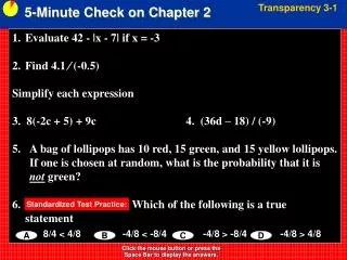
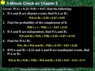
5-Minute Check on Chapter 5 Given: P(A) = 0.25; P(B) = 0.67, find the following: If A and B are disjoint events, find P(A or B). Find the probability of the complement of B. If A and B are independent, find P(A and B). Find the P(A | B). If P(A and B) = 0.21 and A and B are nondisjoint events, find P(A or B). P(A or B) = 0.25 + 0.67 = 0.92 P(Bc) = 1 – P(B) = 1 – 0.67 = 0.33 P(A and B) = P(A) × P(B) = 0.25 × 0.67 = 0.167 P(A | B) = P(A and B) P(B) = 0.167 0.67 = 0.25 P(A or B) = P(A) + P(B) – P(A and B) = 0.25 + 0.67 – 0.21 = 0.71 Click the mouse button or press the Space Bar to display the answers.
Lesson 6 - 1 Discrete and ContinuousRandom Variables
Objectives • APPLY the concept of discrete random variables to a variety of statistical settings • CALCULATE and INTERPRET the mean (expected value) of a discrete random variable • CALCULATE and INTERPRET the standard deviation (and variance) of a discrete random variable • DESCRIBE continuous random variables
Vocabulary • Random Variable – a variable whose numerical outcome is a random phenomenon • Discrete Random Variable – has a countable number of random possible values • Probability Histogram – histogram of discrete outcomes versus their probabilities of occurrence • Continuous Random Variable – has a uncountable number (an interval) of random possible values • Probability Distribution – is a probability density curve
Probability Rules • 0 ≤ P(X) ≤ 1 for any event X • P(S) = 1 for the sample space S • Addition Rule for Disjoint Events: • P(A B) = P(A) + P(B) • Complement Rule: • For any event A, P(AC) = 1 – P(A) • Multiplication Rule: • If A and B are independent, then P(A B) = P(A)P(B) • General Addition Rule (for nondisjoint) Events: • P(E F) = P(E) + P(F) – P(E F) • General Multiplication rule: • P(A B) = P(A) P(B | A)
Probability Terms • Disjoint Events: • P(A B) = 0 • Events do not share any common outcomes • Independent Events: • P(A B) = P(A) P(B) (Rule for Independent events) • P(A B) = P(A) P(B | A) (General rule) • P(B) = P(B|A) (lines 1 and 2 implications) • Probability of B does not change knowing A • At Least One: • P(at least one) = 1 – P(none) • From the complement rule [ P(AC) = 1 – P(A) ] • Impossibility: P(E) = 0 • Certainty: P(E) = 1
Example 1 Write the following in probability format: • Exactly 6 bulbs are red • Fewer than 4 bulbs were blue • At least 2 bulbs were white • No more than 5 bulbs were purple • More than 3 bulbs were green P(red bulbs = 6) P(blue bulbs < 4) P(white bulbs ≥ 2) P(purple bulbs ≤ 5) P(green bulbs > 3)
Random Variable and Probability Distribution A probability model describes the possible outcomes of a chance process and the likelihood that those outcomes will occur. A numerical variable that describes the outcomes of a chance process is called a random variable. The probability model for a random variable is its probability distribution Definition: A random variable takes numerical values that describe the outcomes of some chance process. The probability distribution of a random variable gives its possible values and their probabilities.
Coin Flip Example • Consider tossing a fair coin 3 times. • Define X = the number of heads obtained X = 0: TTT X = 1: HTT THT TTH X = 2: HHT HTH THH X = 3: HHH
Discrete Random Variables • There are two main types of random variables: discrete and continuous. If we can find a way to list all possible outcomes for a random variable and assign probabilities to each one, we have a discrete random variable. Discrete Random Variables and Their Probability Distributions • A discrete random variable X takes a fixed set of possible values with gaps between. The probability distribution of a discrete random variable X lists the values xiand their probabilities pi: • Value: x1x2x3 … • Probability: p1p2p3… • The probabilities pi must satisfy two requirements: • Every probability piis a number between 0 and 1. • The sum of the probabilities is 1. • To find the probability of any event, add the probabilities piof the particular values xithat make up the event.
Discrete Random Variables • Variable’s values follow a probabilistic phenomenon • Values are countable • Examples: • Rolling Die • Drawing Cards • Number of Children born into a family • Number of TVs in a house • Distributions that we will study On AP Test Not on AP • Uniform Poisson • Binomial Negative Binomial • Geometric Hypergeometric
Babies’ Health at Birth Apgar scores measure a baby’s health at birth; rating skin color, heart rate, muscle tone, breathing and stimuli response on a 0-1-2 scale for each category • Show that the probability distribution for X is legitimate. • Make a histogram of the probability distribution. Describe what you see. • Apgar scores of 7 or higher indicate a healthy baby. What is P(X ≥ 7)?
Babies’ Health at Birth • Show that the probability distribution for X is legitimate. • Make a histogram of the probability distribution. Describe what you see. • Apgar scores of 7 or higher indicate a healthy baby. What is P(X ≥ 7)? pi = 1 skewed left P(x ≥ 7) = 0.1+.32+.44+.05 = .908
Discrete Example • Most people believe that each digit, 1-9, appears with equal frequency in the numbers we find
Discrete Example cont • Benford’s Law • In 1938 Frank Benford, a physicist, found our assumption to be false • Used to look at frauds
Example 4 • Verify Benford’s Law as a probability model • Use Benford’s Law to determine • the probability that a randomly selected first digit is 1 or 2 • the probability that a randomly selected first digit is at least 6 Summation of P(x) = 1 P(1 or 2) = P(1) + P(2) = 0.301 + 0.176 = 0.477 P(≥6) = P(6) + P(7) + P(8) + P(9) = 0.067 + 0.058 + 0.051 + 0.046 = 0.222
Example 5 Write the following in probability format with discrete RV (25 colored bulbs): • Exactly 6 bulbs are red • Fewer than 4 bulbs were blue • At least 2 bulbs were white • No more than 5 bulbs were purple • More than 3 bulbs were green P(red bulbs = 6) = P(6) P(blue bulbs < 4) = P(0) + P(1) + P(2) + P(3) P(white bulbs ≥ 2) = P(≥ 2) = 1 – [P(0) + P(1)] P(purple bulbs ≤ 5) = P(0) + P(1) + P(2) + P(3) + P(4) + P(5) P(green bulbs > 3) = P(> 3) = 1 – [P(0) + P(1) + P(2)]
Summary and Homework • Summary • Random variables (RV) values are a probabilistic • RV follow probability rules • Discrete RV have countable outcomes • Homework • Day 1:
5-Minute Check on section 6-1a Convert these statements into discrete probability expressions Probability of less than 4 green bulbs Probability of more than 2 green lights Probability of 3 or more If x is a discrete variable x[1,3], P(x=1) = 0.23, and P(x=2) = 0.3 Find P(x<3) Find P(x=3) Find P(x>1) P(x < 4) = P(0) + P(1) + P(2) + P(3) P(x > 2) = P(3) + P(4) + P(5) + … P(x 3) = P(3) + P(4) + P(5) + … = P(1) + P(2) = 0.23 + 0.3 = 0.57 = 1 – (P(1) + P(2)) = 1 – 0.57 = 0.43 = P(2) + P(3) = 0.3 + 0.43 = 0.73 Click the mouse button or press the Space Bar to display the answers.
Warning! • Statistical analysis is not for the faint of heart
Mean of a Discrete Random Variable When analyzing discrete random variables, we’ll follow the same strategy we used with quantitative data – describe the shape, center, and spread, and identify any outliers. The mean of any discrete random variable is an average of the possible outcomes, with each outcome weighted by its probability. Definition: Suppose that X is a discrete random variable whose probability distribution is Value: x1x2x3 … Probability: p1p2p3 … To find the mean (expected value) of X, multiply each possible value by its probability, then add all the products:
Apgar Scores – What’s Typical? Consider the random variable X = Apgar Score Compute the mean of the random variable X and interpret it in context. The mean Apgar score of a randomly selected newborn is 8.128. This is the long-term average Agar score of many, many randomly chosen babies. Note: The expected value does not need to be a possible value of X or an integer! It is a long-term average over many repetitions.
Standard Deviation of a Discrete Random Variable Since we use the mean as the measure of center for a discrete random variable, we’ll use the standard deviation as our measure of spread. The definition of the variance of a random variable is similar to the definition of the variance for a set of quantitative data. Definition: Suppose that X is a discrete random variable whose probability distribution is Value: x1x2x3 … Probability: p1p2p3 … and that µXis the mean of X. The variance of X is To get the standard deviation of a random variable, take the square root of the variance.
Apgar Scores – How Variable Are They? Consider the random variable X = Apgar Score Compute the standard deviation of the random variable X and interpret it in context. Variance The standard deviation of X is 1.437. On average, a randomly selected baby’s Apgar score will differ from the mean 8.128 by about 1.4 units.
Example 1 You have a fair 10-sided die with the number 1 to 10 on each of the faces. Determine the mean and standard deviation. Mean: ∑ [x ∙P(x)] = (1/10) (∑ x) = (1/10)(55) = 5.5 Var: ∑[x2 ∙ P(x)] – μ2x = (1/n) ∑ [x2 ] – μx2 = (1/10) (385) - 30.25) = (38.5 – 30.25) = 8.25 St Dev = 2.8723
Calculator to the Rescue We can use 1-Var-Stats to calculate the mean and standard deviation of a discrete random variable given it’s outcomes and probability • Type in outcomes (x values) in L1 • Type in corresponding probabilities in L2 • Use 1-Var-Stats L1, L2 to get statistics We can graph the probability histograms by changing the frequency to L2
Example 2 Below is a distribution for number of visits to a dentist in one year. X = # of visits to a dentist x 0 1 2 3 4 P(x) .1 .3 .4 .15 .05 Determine the expected value, variance and standard deviation. Mean: ∑ [x ∙P(x)] = (.1)(0) + (.3)(1) + (.4)(2) + (.15)(3) + (.05)(4) = 0 + .3 + .8 + .45 +.2 = 1.75 Var: ∑[x2 ∙ P(x)] – μ2x = ∑ [x2 ∙ P(x)] – μx2 = (0 + .3 + .4(4) + .15(9) + .05(16) ) – 3.0625) = 4.05 – 3.8626 = 0.9875 St Dev = 0.9937
Example 3 What is the average size of an American family? Here is the distribution of family size according to the 1990 Census: # in family 2 3 4 5 6 7 p(x) .413 .236 .211 .090 .032 .018 Mean: ∑ [x ∙P(x)] = (.413)(2) + (.236)(3) + (.211)(4) + (.09)(5) + (.032)(6) + (.018)(7) = .826 + .708 + .844 + .45 + .192 + .126 = 3.146
Continuous Random Variables Discrete random variables commonly arise from situations that involve counting something. Situations that involve measuring something often result in a continuous random variable. Definition: A continuous random variableX takes on all values in an interval of numbers. The probability distribution of X is described by a density curve. The probability of any event is the area under the density curve and above the values of X that make up the event. The probability model of a discrete random variable X assigns a probability between 0 and 1 to each possible value of X. A continuous random variable Y has infinitely many possible values. All continuous probability models assign probability 0 to every individual outcome. Only intervals of values have positive probability.
Continuous Random Variables • Variable’s values follow a probabilistic phenomenon • Values are uncountable (infinite) • P(X = any value) = 0 (area under curve at a point) • Examples: • Plane’s arrival time -- minutes late (uniform) • Calculator’s random number generator (uniform) • Heights of children (apx normal) • Birth Weights of children (apx normal) • Distributions that we will study • Uniform • Normal
Continuous Random Variables • We will use a normally distributed random variable in the majority of statistical tests that we will study this year • Need to justify it (as a reasonable assumption) if is not given • Normality graphs if we have raw data • We need to be able to • Use z-values in Table A • Use the normalcdf from our calculators • Graph normal distribution curves
Example: Young Women’s Heights Read the example on pg 351. Define Y = height of a randomly chosen young woman. Y is a continuous random variable whose probability distribution is N(64, 2.7). What is the probability that a randomly chosen young woman has height between 68 and 70 inches? P(68 ≤ Y ≤ 70) = ??? Use calculator: normcdf(68,70,64,2.7) or use Z-tables by converting 68 and 72 into z-scores P(68 ≤ Y ≤ 70) = .0562 There is about a 5.6% chance that a randomly chosen young woman has a height between 68 and 70 in.
Example 4 Determine the probability of the following random number generator: • Generating a number equal to 0.5 • Generating a number less than 0.5 or greater than 0.8 • Generating a number bigger than 0.3 but less than 0.7 P(x = 0.5) = 0.0 P(x ≤ 0.5 or x ≥ 0.8) = 0.5 + 0.2 = 0.7 P(0.3 ≤ x ≤ 0.7) = 0.4
Example 5 In a survey the mean percentage of students who said that they would turn in a classmate they saw cheating on a test is distributed N(0.12, 0.016). If the survey has a margin of error of 2%, find the probability that the survey misses the percentage by more than 2% [P(x<0.1 or x>0.14)] Change into z-scores to use table A 0.10 – 0.14 z = ---------------- = +/- 1.25 0.016 0.8944 – 0.1056 = 0.7888 1 – 0.7888 = 0.2112 ncdf(0.1, 0.14, 0.12, 0.016) = 0.7887 1 – 0.7887 = 0.2112
Summary and Homework • Summary • Random variables (RV) values are a probabilistic • RV follow probability rules • Discrete RV have countable outcomes • Continuous RV has an interval of outcomes (∞) • Expected value is the mean ∑ [x ∙ P(x)] • Variance is ∑[x2 ∙ P(x)] – μ2x • Standard Deviation is variance • Homework • Day 2: