Bayesian Hypothesis Testing and Bayes Factors
Bayesian Hypothesis Testing and Bayes Factors. Bayesian p-values Bayes Factors for model comparison Easy to implement alternatives for model comparison. Bayesian Hypothesis Testing. Bayesian hypothesis testing is less formal than non-Bayesian varieties.

Bayesian Hypothesis Testing and Bayes Factors
E N D
Presentation Transcript
Bayesian Hypothesis Testing and Bayes Factors Bayesian p-values Bayes Factors for model comparison Easy to implement alternatives for model comparison
Bayesian Hypothesis Testing Bayesian hypothesis testing is less formal than non-Bayesian varieties. In fact, Bayesian researchers typically summarize the posterior distribution without applying a rigid decision process. Since social scientists don’t actually make important decisions based on their findings, posterior summaries are more than adequate. If one wanted to apply a formal process, Bayesian decision theory is the way to go because it is possible to get a probability distribution over the parameter space and one can make expected utility calculations based on the costs and benefits of different outcomes. Considerable energy has been given, however, in trying to map Bayesian statistical models into the null hypothesis hypothesis testing framework, with mixed results at best.
Similarities between Bayesian and Frequentist Hypothesis Testing • Maximum likelihood estimates of parameter means and standard errors and Bayesian estimates with flat priors are equivalent. • Asymptotically, the data will overwhelm the choice of prior, so if we had infinite data sets, priors would be irrelevant and Bayesian and frequentist results would converge. • Frequentist one-tailed tests are basically equivalent to what a Bayesian would get using credible intervals.
Differences between Frequentist and Bayesian Hypothesis Testing The most important pragmatic difference between Bayesian and frequentist hypothesis testing is that Bayesian methods are poorly suited for two-tailed tests. Why? Because the probability of zero in a continuous distribution is zero. The best solution proposed so far is to calculate the probability that, say, a regression coefficient is in some range near zero. e.g. two sided p-value = Pr(-e < B < e) However, the choice of e seems very ad hoc unless there is some decision theoretic basis. The other important difference is more philosophical. Frequentist p-values violate the likelihood principle.
Bayes FactorsNotes taken from Gill (2002) Bayes Factors are the dominant method of Bayesian model testing. They are the Bayesian analogues of likelihood ratio tests. The basic intuition is that prior and posterior information are combined in a ratio that provides evidence in favor of one model specification verses another. Bayes Factors are very flexible, allowing multiple hypotheses to be compared simultaneously and nested models are not required in order to make comparisons -- it goes without saying that compared models should obviously have the same dependent variable.
The General Form for Bayes Factors Suppose that we observe data X and with to test two competing models—M1 and M2, relating these data to two different sets of parameters, 1 and 2. We would like to know which of the following likelihood specifications is better: M1: f1(x | 1) and M2: f2(x | 1) Obviously, we would need prior distributions for the 1 and 2 and prior probabilities for M1 and M2 The posterior odds ratio in favor of M1 over M2 is: Rearranging terms, we find that the Bayes’ Factor is: If we have nested models and P(M1) = P(M2) = .5, then the Bayes Factor reduces to the likelihood ratio.
Rule of Thumb • With this setup, if we interpret model 1 as the null model, then: • If B(x) 1 then model 1 is supported • If 1 > B(x) 10-1/2 then minimal evidence against model 1. • If 10-1/2 > B(x) 10-1 then substantial evidence against model 1. • If 10-1 > B(x) 10-2 then strong evidence against model 1. • If 10-2 > B(x) then decisive evidence against model 1.
The Bad News Unfortunately, while Bayes Factors are rather intuitive, as a practical matter they are often quite difficult to calculate. Some examples of determining the Bayes Factor in WinBugs for a variable mean can be found in Congdon (example 2.2); and more complex models in Congdon Chapter 10. You also may want to use Carlin and Chib’s technique for computing Bayes Factors for competing non-nested regression models reported in Journal of Royal Statistical Society. Series B. vol 57:3 1995. this technique is implemented in the Pines example in BUGS, and is reported on the Winbugs website under the new examples section. Our discussion will focus on alternatives to the Bayes Factor.
Alternatives to the Bayes Factor for model assessment Let * denote your estimates of the parameter means (or medians or modes) in your model and suppose that the Bayes estimate is approximately equal to the maximum likelihood estimate, then the following stats used in frequentist statistics will be useful diagnostics. Good: The Likelihood Ratio Ratio = -2[log-L(Restricted Model*|y) – log-L(Full Model*|y)] This statistic will always favor the unrestricted model, but when the Bayes estimators or equivalent to the maximum likelihood estimates, then the Ratio is distributed as a 2 where the number of degrees of freedom is equal to the number of test parameters.
Alternatives to the Bayes Factor for model assessment Let * denote your estimates of the parameter means (or medians or modes) in your model and suppose that the Bayes estimate is approximately equal to the maximum likelihood estimate, then the following stats used in frequentist statistics will be useful diagnostics. Better: Akaike Information Criterion (AIC) AIC = -2log-L(*|y) + 2p (where p = the number of parameters including the intercept). To compare two models, compare the AIC from model 1 against the AIC from model 2. Smaller numbers are better. Models do not need to be nested The AIC tends to be biased in favor of more complicated models, because the log-likelihood tends to increase faster than the number of parameters.
Alternatives to the Bayes Factor for model assessment Better still: Bayesian Information Criterion (BIC) BIC = -2log-L(*|y) + 2p*log(n) (where p = the number of parameters and n is the sample size). This statistic can also be used for non-nested models BIC1 – BICl2 the -2 log(Bayes Factor12) for model 1 vs. model 2.
Alternatives to the Bayes Factor for model assessment Best ??? : Deviance Information Criterion (DIC) This is a new statistic introduced by the developers of WinBugs (and can therefore be reported in WinBugs!). Spiegelhalter, et al. 2002. “Bayesian measures of model complexity and fit.” Journal of the Royal Statistical Society Series B. pp. 583-639. It is not an approximation of the Bayes Factor! DIC = Mean[ -2log-L(t|y) ] – { Mean[-2log-L(t|y)] - 2log-L(*|y) } This is the Deviance (DBar): it is the average of the log-likelihoods calculated at the end of an iteration of the Gibbs Sampler. This (Dhat) is the log-likelihood calculated using the posterior means of The second expression (Dbar - Dhat = pD) is the penalty for over-parameterizing the model. To see this, note that having a lot of insignificant parameters with large variances will yield iterations of the Gibbs Sampler with likelihoods far from Dhat.
Example—Predictors of International Birth Rates, 2000 Dependent Variable: - Births per female Independent Variables: - GDP Growth Rate - Female Illiteracy - Dependents / Working Age Population Probability Model: Births ~ N(b0 + b1 GDP + b2 Illiteracy + b3 AgeDep + b4, t) bj ~ N(0, .001) for all j and t ~ G(.001,.001) The Null Model: Births ~ N(a , tnull) a ~ N(0, .001) and tnull ~ G(.001,.001)
WinBugs Code model { for (i in 1:150) { birthrate[i] ~ dnorm(mu[i], tau) mu[i] <- b[1]*gdprate[i] + b[2]*femillit[i] + b[3]*agedep[i] + b[4] } for (j in 1:4) { b[j] ~ dnorm(0, .0001) } tau ~ dgamma(.001,.001) # code to create a null model for (i in 1:150) { null[i] <- birthrate[i] null[i] ~ dnorm(mu2[i], tau2) mu2[i] <- a } a ~ dnorm(0,.0001) tau2 ~ dgamma(.001,.001) } Inits: list(tau = 1, tau2 = 1); list(tau = 100, tau2=100)
Results node mean sd MC error a 3.119 0.133 0.002157 tau2 0.369 0.043 5.977E-4 gdprate 0.011 0.016 2.499E-4 femillit 0.014 0.004 5.137E-5 agedep 6.581 0.519 0.007473 intercept -1.537 0.301 0.004301 tau 1.943 0.226 0.003065 Deviance 903.4 3.844 0.05402 (Sum for Null model deviance and Full Model) Null Model Full Model Dbar = post.mean of -2logL; Dhat = -2LogL at post.mean of stochastic nodes Dbar Dhat pD DIC full 327.145 322.104 5.041 332.186 null 576.221 574.244 1.977 578.198 total 903.366 896.348 7.018 910.384
Results Dbar = post.mean of -2logL; Dhat = -2LogL at post.mean of stochastic nodes Dbar Dhat pD DIC full 327.145 322.104 5.041 332.186 null 576.221 574.244 1.977 578.198 total 903.366 896.348 7.018 910.384 Let Dhat = -2LogL(*) Then we can implement each of the three diagnostic tests. Likelihood Ratio = -2[log-L(Null*|y) – log-L(Full*|y)] = 574.244 - 322.104 252 ~ 23 reject null model AICnull = -2log-L(null*|y) + 2p = 574.244 + 2*1 = 576 AICfull = -2log-L(full*|y) + 2p = 332.186 + 2*4 = 340 favors full BICnull = -2log-L(null*|y) + 2plog(n) = 574.244 + 2*1*log(150) = 584 BICfull= -2log-L(full*|y) + 2plog(n) = 332.186 + 2*4*log(150) = 370 favors full DICnull = 578.198 DICfull = 332.186
Calculating MSE and R2 in WinBugs Mean Squared Error and the R2 are two very common diagnostics for regression models. Calculating these quantities in WinBugs is rather straightforward if we monitor nodes programmed to calculate these statistics just like the deviance statistic is a monitored value of the likelihood. Recall that: MSE = i ( yi – pred(yi) )2 / n and R2 = i ( pred(yi) – mean(y) )2 / i ( yi – mean(y) )2 and note that in WinBugs-Speak: pred(yi) = mu[i] model { for (i in 1:150) { birthrate[i] ~ dnorm(mu[i], tau) mu[i] <- b[1]*gdprate[i] + b[2]*femillit[i] + b[3]*agedep[i] + b[4] numerator[i] <- (mu[i]-mean(birthrate[]))*(mu[i]-mean(birthrate[])) denominator[i] <- (birthrate[i]-mean(birthrate[]))*(netft[i]-mean(birthrate[])) se[i] <- (mu[i]-birthrate[i])*(mu[i]-birthrate[i]) } for (j in 1:4) { b[j] ~ dnorm(0, .0001) } tau ~ dgamma(.001,.001) R2 <- sum(numerator[])/sum(denominator[]) SSE <- sum(se[]) MSE <- mean(se[]) }
A final diagnostic Researchers should always check residual plots in a linear regression model to see if the errors are approximately normal. In WinBugs, if the likelihood function is specified in the following way: y[i] ~ dnorm(mu[i] , tau) You may set the sample monitor to mu. This will monitor the expected value of your dependent variable given the regression coefficients.