Download
1 / 31
350 likes | 833 Vues
Special Inventory Models. Supplement D. Special Inventory Models. Three common situations require relaxation of one or more of the assumptions on which the EOQ model is based.

E N D
Special Inventory Models Supplement D
Special Inventory Models • Three common situations require relaxation of one or more of the assumptions on which the EOQ model is based. • Noninstantaneous Replenishment occurs when production is not instantaneous and inventory is replenished gradually, rather than in lots. • Quantity Discounts occur when the unit cost of purchased materials is reduced for larger order quantities. • One-Period Decisions: Retailers and manufacturers of fashion goods often face situations in which demand is uncertain and occurs during just one period or season.
Noninstantaneous Replenishment • If an item is being produced internally rather than purchased, finished units may be used or sold as soon as they are completed, without waiting until a full lot is completed. • Production rate, p, exceeds the demand rate, d. • Cycle inventory accumulates faster than demand occurs • a buildup of p – d units occurs per time period, continuing until the lot size, Q, has been produced.
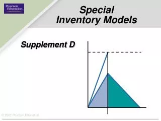
Production quantity Q Demand during production interval Imax On-hand inventory Maximum inventory p – d Time Production and demand Demand only TBO Noninstantaneous Replenishment
Imax = (p – d) = Q( ) Q p C = ( ) + (S) p – d p Q p – d 2 p D Q Noninstantaneous Replenishment • Cycle inventory is no longer Q/2, as it was with the basic EOQ method; instead, it is the maximum cycle inventory (Imax/ 2) • Total annual cost (C) = Annual holding cost + annual ordering or setup cost D = annual demandd = daily demandp = production rateS = setup costs Q = ELS
p p – d 2DS H ELS = Economic Lot Size (ELS) • Economic production lot size (ELS) is the optimal lot size in a situation in which replenishment is not instantaneous. D = annual demandd = daily demandp = production rateS = setup costs H = annual unit holding cost
Demand = 30 barrels/day Setup cost = $200 Production rate = 190 barrels/day Annual holding cost = $0.21/barrel Annual demand = 10,500 barrels Plant operates 350 days/year Finding the ELS Example D.1 The manager of a chemical plant must determine the following for a particular chemical: • Determine the economic production lot size (ELS). • Determine the total annual setup and inventory holding costs. • Determine the TBO, or cycle length, for the ELS. • Determine the production time per lot. • What are the advantages of reducing the setup time by 10 percent?
2(10,500)($200) $0.21 190 190 – 30 ELS = p p – d 2DS H ELS = Demand = 30 barrels/day Setup cost = $200 Production rate = 190 barrels/day Annual holding cost = $0.21/barrel Annual demand = 10,500 barrels Plant operates 350 days/year Finding the ELS for the Example D.1 chemical D = annualdemandd = dailydemandp = productionrateS = setupcosts H = unitholdingcost Q = ELS ELS = 4873.4 barrels
C = ( )(H) + (S) C = ( ) ($0.21) + ($200) Q p – d 2 p D Q 10,500 4873.4 4873.4 190 – 30 2 190 Demand = 30 barrels/day Setup cost = $200 Production rate = 190 barrels/day Annual holding cost = $0.21/barrel Annual demand = 10,500 barrels Plant operates 350 days/year Finding the Total Annual Cost Example D.1 D = annualdemandd = dailydemandp = productionrateS = setupcosts H = unitholdingcost Q = ELS C = $430.91 + $430.91 C = $861.82
4873.4 10,500 ELS D Demand = 30 barrels/day Setup cost = $200 Production rate = 190 barrels/day Annual holding cost = $0.21/barrel Annual demand = 10,500 barrels Plant operates 350 days/year TBOELS = (350 days/year) TBOELS = (350 days/year) Finding the TBO Example D.1 D = annual demandd = dailydemandp = productionrateS = setupcosts H = unitholdingcost Q = ELS TBOELS = 162.4, or 162 days
4873.4 190 ELS p Production time = Production time = Demand = 30 barrels/day Setup cost = $200 Production rate = 190 barrels/day Annual holding cost = $0.21/barrel Annual demand = 10,500 barrels Plant operates 350 days/year Finding the Production Time per Lot Example D.1 D = annual demandd = daily demandp = production rateS = setupcosts H = unitholdingcost Q = ELS Production time = 25.6, or 26 days
Advantage of Reducing Setup Time OM Explorer Solver for the Economic Production Lot Size Showing the effect of a 10 Percent Reduction in setup cost. $180 vs original $200
Application D.1 or 1555 engines
D Q Q 2 C = (H) + (S) + PD Quantity Discounts • Quantity discounts, which are price incentives to purchase large quantities, create pressure to maintain a large inventory. • For any per-unit price level, P, the total cost is: • Total annual cost = Annual holding cost + Annual ordering or setup cost + Annual cost of materials D = annual demandS = setup costsP = per-unit price level H = unit holding cost Q = ELS
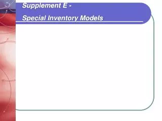
EOQ 4.00 EOQ 3.50 EOQ 3.00 C for P = $4.00 C for P = $3.50 C for P = $3.00 Total cost (dollars) PD for P = $4.00 Total cost (dollars) PD for P = $3.50 PD for P = $3.00 First price break Second price break First price break Second price break 0 100 200 300 0 100 200 300 Purchase quantity (Q) Purchase quantity (Q) Quantity Discounts Total cost curves with purchased materials added EOQs and price break quantities
Finding Q with Quantity Discounts • Step 1. Beginning with the lowest price, calculate the EOQ for each price level until a feasible EOQ is found. • It is feasible if it lies in the range corresponding to its price. • Step 2. If the first feasible EOQ found is for the lowest price level, this quantity is the best lot size. • Otherwise, calculate the total cost for the first feasible EOQ and for the larger price break quantity at each lower price level. The quantity with the lowest total cost is optimal.
Order Quantity Price per Unit 0 – 299 $60.00 300 – 499 $58.80 500 or more $57.00 2DS H EOQ 57.00 = 2(936)(45) 0.25(57.00) = 77 units = Example D.2 A supplier for St. LeRoy Hospital has introduced quantity discounts to encourage larger order quantities of a special catheter. The price schedule is: Annual demand (D) = 936 units Ordering cost (S) = $45 Holding cost (H) = 25% of unit price Step 1: Start with lowest price level:
Order Quantity Price per Unit 0 – 299 $60.00 300 – 499 $58.80 500 or more $57.00 2DS H 2DS H 2DS H EOQ 57.00 = EOQ 58.80 = EOQ 60.00 = 2(936)(45) 0.25(58.80) 2(936)(45) 0.25(57.00) 2(936)(45) 0.25(60.00) = 76 units = 75 units = 77 units = = = Example D.2continued Not feasible Not feasible Feasible This quantity is feasible because it lies in the range corresponding to its price. Annual demand (D) = 936 units Ordering cost (S) = $45 Holding cost (H) = 25% of unit price
= $57,382 = $56,999 936 75 75 2 C75 = [(0.25)($60.00)] + ($45) + $60.00(936) D Q Q 2 C = (H) + (S) + PD 936 300 300 2 C300 = [(0.25)($58.80)] + ($45) + $58.80(936) 936 500 500 2 C500 = [(0.25)($57.00)] + ($45) + $57.00(936) Example D.2continued • Step 2: The first feasible EOQ of 75 does not correspond to the lowest price level. Hence, we must compare its total cost with the price break quantities (300 and 500 units) at the lower price levels ($58.80 and $57.00): C75 = $57,284 The best purchase quantity is 500 units, which qualifies for the deepest discount.
© 2007 Pearson Education Decision Point: If the price per unit for the range of 300 to 499 units is reduced to $58.00, the best decision is to order 300 catheters, as shown below. This shows that the decision is sensitive to the price schedule. A reduction of slightly more than 1 percent is enough to make the difference in this example.
One-Period Decisions • This type of situation is often called the newsboy problem. If the newspaper seller does not buy enough newspapers to resell on the street corner, sales opportunities are lost. If the seller buys too many newspapers, the overage cannot be sold because nobody wants yesterday’s newspaper. • List the different levels of demand that are possible, along with the estimated probability of each. • Develop a payoff table that shows the profit for each purchase quantity, Q, at each assumed demand level. • Calculate the expected payoff for each Q (or row in the payoff table) by using the expected value decision rule. • Choose the order quantity Q with the highest expected payoff.
One-Period Decisions • The payoff for a given quantity-demand combination depends on whether all units are sold at the regular profit margin, which results in two possible cases. • If demand is high enough (Q <D) then all of the cases are sold at the full profit margin, p, during the regular season. Payoff = (Profit per unit)(Purchase quantity) = pQ • If the purchase quantity exceeds the eventual demand (Q > D), only D units are sold at the full profit margin, and the remaining units purchased must be disposed of at a loss, l, after the season. Payoff = (Profit per unit during season) (Demand) – (Loss per unit) (Amount disposed of after season) = pD – l(Q – D)
Demand 10 20 30 40 50 Demand Probability 0.2 0.3 0.3 0.1 0.1 Q 10 20 30 40 50 Expected Payoff 10 $100 $100 $100 $100 $100 100 20 50 200 200 200 200 170 30 0 150 300 300 300 195 40 –50 100 250 400 400 175 50 –100 50 200 350 500 140 Payoff if Q = 30 and D = 40: pD = 10(30) = $300 Payoff if Q = 30 and D = 20: pD – l(Q – D)=10(20) – 5(30 – 20) = $150 Expected payoff if Q = 30: 0(0.2)+(150(0.3)+300(0.3+0.1+0.1) = $195 © 2007 Pearson Education Example D.3 A gift museum shop sells a Christmas ornament at a $10 profit per unit during the holiday season, but it takes a $5 loss per unit after the season is over. The following is the discrete probability distribution for the season’s demand:
© 2007 Pearson Education Example D.3 OM Explorer Solution
Solved Problem 1 • For Peachy Keen, Inc., the average demand for mohair sweaters is 100 per week. The production facility has the capacity to sew 400 sweaters per week. Setup cost is $351. The value of finished goods inventory is $40 per sweater. The annual per-unit inventory holding cost is 20 percent of the item’s value. • a. What is the economic production lot size (ELS)? • b. What is the average time between orders (TBO)? • c. What is the minimum total of the annual holding cost and setup cost?
= 780 sweaters 400 (400 – 100) 2(100)(52)($351) 0.20($40) ELS = p p – d 2DS H ELS = 780 5,200 C = ( )(H) + (S) = = 0.15 year or 7.8 weeks Q p – d 2 p D Q C = ( ) (0.20 x $40) + ($351) 5,200 780 780 400 – 100 2 400 ELS D TBOELS = = 2,340/year + $2,340/year = $4,680/year © 2007 Pearson Education Solved Problem 1 a. D = 5,200p = 400 d = 100S = $351 H= 20% of $40 b. c.
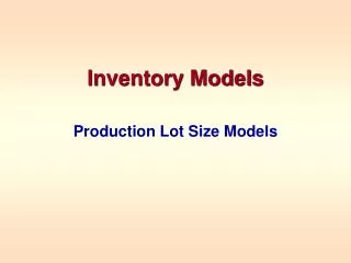
Solved Problem 3 • For Swell Productions, a concession stand will sell poodle skirts and other souvenirs of the 1950s a one-time event. Skirts are purchased for $40 each and are sold during for $75 each. • Unsold skirts can be returned for a refund of $30 each. Sales depend on the weather, attendance, and other variables. • The following table shows the probability of various sales quantities. How many skirts should be ordered?
0.05 0.11 0.34 0.34 0.11 0.05 Probabilities Solved Problem 3 The highest expected payoff occurs when 400 skirts are ordered.