Autoregressive Integrated Moving Average (ARIMA) models
Autoregressive Integrated Moving Average (ARIMA) models. - Forecasting techniques based on exponential smoothing General assumption for the above models: times series data are represented as the sum of two distinct components ( deterministc & random)

Autoregressive Integrated Moving Average (ARIMA) models
E N D
Presentation Transcript
- Forecasting techniques based on exponential smoothing • General assumption for the above models: times series data are represented as the sum of two distinct components (deterministc & random) • Random noise: generated through independent shocks to the process • In practice: successive observations show serial dependence
ARIMA Models - ARIMA models are also known as the Box-Jenkins methodology • very popular : suitable for almost all time series & many times generate more accurate forecasts than other methods. • limitations: • If there is not enough data, they may not be better at forecasting than the decomposition or exponential smoothing techniques. • Recommended number of observations at least 30-50 • - Weak stationarity is required • - Equal space between intervals
Linear Filter • - It is a process that converts the input xt, into output yt • The conversion involves past, current and future values of the input in the form of a summation with different weights • Time invariant do not depend on time • Physically realizable: the output is a linear function of the current and past values of the input • Stable if In linear filters: stationarity of the input time series is also reflected in the output
A time series that fulfill these conditions tends to return to its mean and fluctuate around this mean with constant variance. Note: Strict stationarity requires, in addition to the conditions of weak stationarity, that the time series has to fulfill further conditions about its distribution including skewness, kurtosis etc. Determine stationarity -Take snaphots of the process at different time points & observe its behavior: if similar over time then stationary time series -A strong & slowly dying ACF suggests deviations from stationarity
Infinite Moving Average Input xt stationary Output yt Stationary, with & THEN, the linear process with white noise time series εt Is stationary εt independent random shocks, with E(εt)=0 &
autocovariance function Linear Process Infinite moving average
The infinite moving average serves as a general class of models for any stationary time series THEOREM (World 1938): Any no deterministic weakly stationary time series yt can be represented as where INTERPRETATION A stationary time series can be seen as the weighted sum of the present and past disturbances
Infinite moving average: • Impractical to estimate the infinitely weights • Useless in practice except for special cases: • i. Finite order moving average (MA) models : weights set to 0, except for a finite number of weights • ii. Finite order autoregressive (AR) models: weights are generated using only a finite number of parameters • iii. A mixture of finite order autoregressive & moving average models (ARMA)
Finite Order Moving Average (MA) process Moving average process of order q(MA(q)) MA(q) : always stationary regardless of the values of the weights
εt white noise Expected value of MA(q) Variance of MA(q) Autocovariance of MA(q) Autocorelation of MA(q)
ACF function: Helps identifying the MA model & its appropriate order as its cuts off after lag k Real applications: r(k) not always zero after lag q; becomes very small in absolute value after lag q
First Order Moving Average Process MA(1) q=1 Autocovariance of MA(q) Autocorelation of MA(q)
Mean & variance : stable • Short runs where successive observations tend to follow each other • Positive autocorrelation • Observations oscillate successively • negative autocorrelation
Second Order Moving Average MA(2) process Autocovariance of MA(q) Autocorelation of MA(q)
Finite Order Autoregressive Process • World’s theorem: infinite number of weights, not helpful in modeling & forecasting • Finite order MA process: estimate a finite number of weights, set the other equal to zero • Oldest disturbance obsolete for the next observation; only finite number of disturbances contribute to the current value of time series • Take into account all the disturbances of the past : • use autoregressive models; estimate infinitely many weights that follow a distinct pattern with a small number of parameters
First Order Autoregressive Process, AR(1) Assume : the contributions of the disturbances that are way in the past are small compared to the more recent disturbances that the process has experienced Reflect the diminishing magnitudes of contributions of the disturbances of the past,through set of infinitely many weights in descending magnitudes , such as Exponential decay pattern The weights in the disturbances starting from the current disturbance and going back in the past:
First order autoregressive process AR(1) where WHY AUTOREGRESSIVE ? AR(1) stationary if
Mean AR(1) Autocovariance function AR(1) Autocorrelation function AR(1) The ACF for a stationary AR(1) process has an exponential decay form
Observe: • The observations exhibit up/down movements
Second Order Autoregressive Process, AR(2) This model can be represented in the infinite MA form & provide the conditions of stationarity for yt in terms of φ1& φ2 WHY? 1. Infinite MA Apply
Calculate the weights We need
Solutions The satisfy the second-order linear difference equation The solution : in terms of the 2 roots m1 and m2 from AR(2) stationary: Condition of stationarity for complex conjugates a+ib: AR(2) infinite MA representation:
Mean Autocovariance function For k=0: Yule-Walker equations For k>0:
Autocorrelation function Solutions A. Solve the Yule-Walker equations recursively B. General solution Obtain it through the roots m1 & m2 associated with the polynomial
Case I: m1, m2 distinct real roots c1, c2 constants: can be obtained from ρ(0) ,ρ(1) stationarity: ACF form: mixture of 2 exponentially decay terms e.g. AR(2) model It can be seen as an adjusted AR(1) model for which a single exponential decay expression as in the AR(1) is not enough to describe the pattern in the ACF and thus, an additional decay expression is added by introducing the second lag term yt-2
Case II: m1, m2 complex conjugates in the form c1, c2: particular constants ACF form: damp sinusoid; damping factor R; frequency ; period
Case III: one real root m0; m1= m2=m0 ACF form: exponential decay pattern
AR(2) process :yt=4+0.4yt-1+0.5yt-2+et Roots of the polynomial: real ACF form: mixture of 2 exponential decay terms
AR(2) process: yt=4+0.8yt-1-0.5yt-2+et Roots of the polynomial: complex conjugates ACF form: damped sinusoid behavior
General Autoregressive Process, AR(p) Consider a pth order AR model or
AR(P) stationary If the roots of the polynomial are less than 1 in absolute value AR(P) absolute summable infinite MA representation Under the previous condition
ACF pth order linear difference equations AR(p) : -satisfies the Yule-Walker equations -ACF can be found from the p roots of the associated polynomial e.g. distinct & real roots : - In general the roots will not be real ACF : mixture of exponential decay and damped sinusoid
ACF • MA(q) process: useful tool for identifying order of process • cuts off after lag k • AR(p) process: mixture of exponential decay & damped sinusoid expressions • Fails to provide information about the order of AR
Partial Autocorrelation Function • Consider : • three random variables X, Y, Z & • Simple regression of X on Z & Y on Z The errors are obtained from
Partial correlation between X & Y after adjusting for Z: The correlation between X* & Y* Partial correlation can be seen as the correlation between two variables after being adjusted for a common factor that affects them
Partial autocorrelation function (PACF) between yt & yt-k The autocorrelation between yt & yt-k after adjusting for yt-1, yt-2, …yt-k AR(p) process: PACF between yt & yt-k for k>p should equal zero • Consider • a stationary time series yt; not necessarily an AR process • For any fixed value k , the Yule-Walker equations for the ACF of an AR(p) process
Matrix notation Solutions For any given k, k =1,2,… the last coefficient is called the partial autocorrelation coefficient of the process at lag k AR(p) process: Identify the order of an AR process by using the PACF
MA(1) MA(2) Decay pattern Decay pattern AR(1) AR(1) Cuts off after 1st lag AR(2) AR(2) Cuts off after 2nd lag
Invertibility of MA models Invertible moving average process: The MA(q) process is invertible if it has an absolute summable infinite AR representation It can be shown: The infinite AR representation for MA(q)