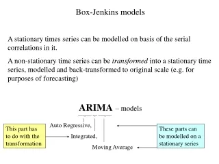
Autoregressive Integrated Moving Average (ARIMA)
Autoregressive Integrated Moving Average (ARIMA) . P opularly known as the Box-Jenkins methodology.

Autoregressive Integrated Moving Average (ARIMA)
E N D
Presentation Transcript
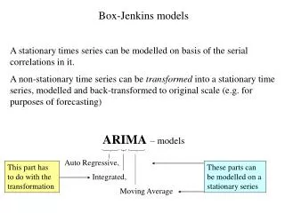
Autoregressive Integrated Moving Average (ARIMA) Popularly known as the Box-Jenkins methodology
ARIMA methodology emphasis not only on constructing single-equation or simultaneous-equation models but also on analyzing the probabilistic or stochastic properties of economic time series on their own set of data. • Unlike the regression models, in which Yi is explained by k regressor X1, X2, X3, ... , Xk the BJ-type time series models allow Yi to be explained by past, or lagged, values of Y itself and stochastic error terms. • For this reason, ARIMA models are sometimes called a theoretic model because they are not derived from any economic theory and economic theories are often the basis of simultaneous-equation models. • Note that the emphasis in this topic is on univariate ARIMA models, as this is pertaining to a single time series. • But can be extended to multivariate ARIMA models.
Let us work with the GDP time series data for the United States given in Table. • A plot of this time series is given in Figures1 (undifferenced GDP) and 2 (first-differenced GDP) • GDP in level form is nonstationary but in (first) differenced form it is stationary. • If a time series is stationary, then it can fit for ARIMA model in a variety of ways. • An Autoregressive (AR) Process • Let Yt represent GDP at time t. • If we model Yt as (Yt - δ) = α1 (Yt-1 – δ) + ut • where δ is the mean of Y and where ut is an uncorrelated random error term with zero mean and constant variance σ2 (i.e., it is white noise), then we say that Yt follows a first-order autoregressive, or AR(l), stochastic process
Here the value of Y at time t depends on its value in the previous time period and a random term; the Y values are expressed as deviations from their mean value. • In other words, this model says that the forecast value of Y at time t is simply some proportion (=αl) of its value at time (t-1) plus a random shock or disturbance at time t; again the Y values are expressed around their mean values. • But in the model, (Yt - δ) = α1 (Yt-1 – δ) + α2 (Yt-2 – δ) + ut • Yt follows a second-order autoregressive, or AR(2), process. • The value of Y at time t depends on its value in the previous two time periods, the Y values being expressed around their mean value δ. • In general, (Yt - δ) = α1 (Yt-1 – δ) + α2 (Yt-2 – δ) + …….. + αp (Yt-p – δ) + ut • Here Yt is a pth order autoregressive or AR(p), process.
A Moving Average (MA) Process • Suppose we model Y as follows: Yt = μ + β0ut + β1ut-1 • where μ is a constant and ut as before, is the white noise stochastic error term. • Here Y at time t is equal to a constant plus a moving average of the current and past error terms. • Thus, in the present case, Y follows a first-order moving average, or an MA(1), process. • But if Y follows the expression Yt = μ + β0ut + β1ut-1 + β2ut-2 then it is an MA(2) process. • Generally, Yt = μ + β0ut + β1ut-1 + β2ut-2 + …….. + βqut-q is an MA(q) process. • In short, a moving average process is simply a linear combination of white noise error terms.
An Autoregressive and Moving Average (ARMA) Process • It is quite likely that Y has characteristics of both AR and MA and is therefore ARMA. • Thus, Yt follows an ARMA (1, 1) process if it can be written as Yt = θ + α1 Yt-1 + β0ut + β1ut-1 • because there is one autoregressive and one moving average term and θ represents a constant term. • In general, in an ARMA (p, q) process, there will be p autoregressive and q moving average terms. • An Autoregressive Integrated Moving Average (ARIMA) Process • Many economic time series are nonstationary, that is, they are integrated.
If a time series is integrated of order 1 [i.e., it is I(1)], its first differences are I(0), that is, stationary. • Similarly, if a time series is I(2), its second difference is I(0). • In general, if a time series is I(d), after differencing it d times we obtain an I(0) series. • Therefore, if in a time series d times difference make it stationary, then it is ARIMA (p, d, q) model is called an autoregressive integrated moving average time series model. • where p denotes the number of autoregressive terms, d the number of times the series has to be differenced before it becomes stationary, and q the number of moving average terms. • An ARIMA(2,1,2) time series has to be differenced once (d =1) becomes stationary and it has two AR and two MA terms.
The important point to note is that to use the Box-Jenkins methodology, we must have either a stationary time series or a time series that is stationary after one or more differencing. • Reason for assuming stationarity can be explained as follows: • The objective of B-J [Box-Jenkins] is to identify and estimate a statistical model which can be interpreted as having generated the sample data. • If this estimated model is then to be used for forecasting we must assume that the features of this model are constant through time, and particularly over future time periods. • Thus the reason for requiring stationary data is that any model which is inferred from these data can itself be interpreted as stationary or stable, therefore providing valid basis for forecasting.
THE BOX-JENKINS (BJ) METHODOLOGY • Looking at a time series, such as the US GDP series in Figure. • How does one know whether it follows a purely AR process (and if so, what is the value of p) or a purely MA process (and if so, what is the value of q) or an ARMA process (and if so, what are the values of p and q) or an ARIMA process. • In which case we must know the values of p, d, and q. • The BJ methodology answering these questions. • The method consists of four steps: • Step 1. Identification: That is, find out the appropriate values of p, d, and q using correlogram and partial correlogram and Augmented Dickey Fuller Test.
Step 2. Estimation: Having identified the appropriate p and q values, the next stage is to estimate the parameters of the autoregressive and moving average terms included in the model. • Sometimes this calculation can be done by simple least squares but sometimes we will have to resort to nonlinear (in parameter) estimation methods. • Since this task is now routinely handled by several statistical packages, we do not have to worry about the actual mathematics of estimation. • Step 3. Diagnostic checking: Having chosen a particular ARIMA model and having estimated its parameters, we next see whether the chosen model fits the data reasonably well, for it is possible that another ARIMA model might do the job as well.
This is why Box-Jenkins ARIMA modeling is more an art than a science; considerable skill is required to choose the right ARIMA model. • One simple test of the chosen model is to see if the residuals estimated from this model are white noise; if they are, we can accept the particular fit; if not, we must start over. • Thus, the BJ methodology is an iterative process. • Step 4. Forecasting: One of the reasons for popularity of the ARIMA modeling is its success in forecasting. • In many cases, the forecasts obtained by this method are more reliable than those obtained from the traditional econometric modeling, particularly for short-term forecasts. • Let us look at these four steps in some detail. Throughout, we will use the GDP data given in Table .
IDENTIFICATION • The chief tools in identification are the autocorrelation function (ACF), the partial autocorrelation function (PACF), and the resulting correlogram, which are simply the plots of ACFs and PACFs against the lag length. • The concept of partial autocorrelation is analogous to the concept of partial regression coefficient. • In the k-variable multiple regression model, the kth regression coefficient βk measures the rate of change in the mean value of the regress and for a unit change in the kth regressor Xk, holding the influence of all other regressors constant.
In similar fashion the partial autocorrelation ρkk measures correlation between (time series) observations that are k time periods apart after controlling for correlations at intermediate lags (i.e., lag less than k). • In other words, partial autocorrelation is the correlation between Yt and Yt-k after removing the effect of intermediate Y's. • In Figure, we show the correlogram and partial correlogram of the GDP series. • From this figure, two facts stand out: • First, the ACF declines very slowly and ACF up to 23 lags are individually statistically significantly different from zero, for they all are outside the 95% confidence bounds. • Second, after the first lag, the PACF drops dramatically, and all PACFs after lag 1 are statistically insignificant.
Since the US GDP time series is not stationary, we have to make it stationary before we can apply the Box-Jenkins methodology. • In next Figure we plotted the first differences of GDP. • Unlike previous Figure, we do not observe any trend in this series, perhaps suggesting that the first-differenced GDP time series is stationary. • A formal application of the Dickey-Fuller unit root test shows that that is indeed the case. • Now we have a different pattern of ACF and PACE The ACFs at lags 1, 8, and 12 seem statistically different from zero. • Approximate 95% confidence limits for ρk are -0.2089 and +0.2089. • But at all other lags are not statistically different from zero. • This is also true of the partial autocorrelations .
Now how do the correlogram given in Figure enable us to find the ARMA pattern of the GDP time series? • We will consider only the first differenced GDP series because it is stationary. • One way of accomplishing this is to consider the ACF and PACF and the associated correlogram of a selected number of ARMA processes, such as AR(l), AR(2), MA(1), MA(2), ARMA(1, 1), ARIMA(2, 2), and so on. • Since each of these stochastic processes exhibits typical patterns of ACF and PACF, if the time series under study fits one of these patterns we can identify the time series with that process. • Of course, we will have to apply diagnostic tests to find out if the chosen ARMA model is reasonably accurate.
What we plan to do is to give general guidelines (see Table ); the references can give the details of the various stochastic processes. • The ACFs and PACFs of AR(p) and MA(q) processes have opposite patterns; in AR(p) case the AC declines geometrically or exponentially but the PACF cuts off after a certain number of lags, whereas the opposite happens to an MA(q) process.
ARIMA Identification of US GDP: • The correlogram and partial correlogram of the stationary (after first-differencing) US GDP for 1970-1 to 1991-IV given in Figure shown • The autocorrelations decline up to lag 4, then except at lags 8 and 12, the rest of them are statistically not different from zero (the solid lines shown in this figure give the approximate 95% confidence limits). • The partial autocorrelations with spikes at lag 1, 8, and 12 seem statistically significant but the rest are not; if the partial correlation coefficient were significant only at lag 1, we could have identified this as an AR (l) model. • Let us therefore assume that the process that generated the (first-differenced) GDP is at the most an AR (12) process. • We do not have to include all the AR terms up to 12, only the AR terms at lag 1, 8, and 12 are significant.
ESTIMATION OFTHE ARIMA MODEL • Let denote the first differences of US GDP. • Then our tentatively identified AR model is • Using Eviews, we obtained the following estimates: • t = (7.7547) (3.4695) (-2.9475) (-2.6817) • R2 = 0.2931 d = 1.7663
DIAGNOSTIC CHECKING • How do we know that the above model is a reasonable fit to the data? • One simple diagnostic is to obtain residuals from the above model and obtain ACF and PACF of these residuals, say, up to lag 25. • The estimated AC and PACF are shown in Figure. • As this figure shows, none of the autocorrelations and partial autocorrelations is individually statistically significant. • Nor is the sum of the 25 squared autocorrelations, as shown by the Box-Pierce Q and Ljung-Box LB statistics statistically significant. • Correlogram of autocorrelation and partial autocorrelation give that the residuals estimated from are purely random. Hence, there may not be any need to look for another ARIMA model.
FORECASTING • Suppose, on the basis of above model, we want to forecast GDP for the first four quarters of 1992. • But in the above model the dependent variable is change in the GDP over the previous quarter. • Therefore, if we use the above model, what we can obtain are the forecasts of GDP changes between the first quarter of 1992 and the fourth quarter of 1991, second quarter of 1992 over the first quarter of 1992, etc. • To obtain the forecast of GDP level rather than its changes, we can "undo" the first-difference transformation that we had used to obtain the changes. • (More technically, we integrate the first-differenced series.)
To obtain the forecast value of GDP (not ΔGDP) for 1992-1, we rewrite model as • Y1992,I - Y1991,IV = δ + αl[Y1991,IV – Y1991,III] + α8[Y1989,IV – Y1989,III] + α12[Y1988,IV – Y1988,III] + u1992-I • That is, Y1992,I = δ + (1+αl)Y1991,IV – αlY1991,III + α8Y1989,IV – α8Y1989,III + α12Y1988,IV – α12Y1988,III + u1992-I • The values of δ , αl, α8, and α12 are already known from the estimated regression. • The value of u1992-I is assumed to be zero. • Therefore, we can easily obtain the forecast value of Y1992-I.
The numerical estimate of this forecast value is • Y1992,I = 23.0894 + (1+0.3428) Y1991,IV - 0.3428 Y1991,III + (-0.2994) Y1989,IV - (-0.2994) Y1989,III + (-0.2644) Y1988,IV – (-0.2644) Y1988,III + u1992-I • = 23.0894 + 1.3428 (4868) - 0.3428 (4862.7) - 0.2994 (4859.7) + 0.2994 (4845.6) - 0.2644 (4779.7) + 0.2644 (4734.5) = 4876.7 • Thus the forecast value of GDP for 1992-I is about $4877 billion (1987 dollars). • The actual value of real GDP for 1992-I was $4873.7 billion; the forecast error was an overestimate of $3 billion.