Auto Regressive, Integrated, Moving Average
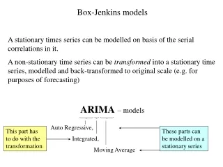
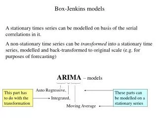
Box-Jenkins models A stationary times series can be modelled on basis of the serial correlations in it. A non-stationary time series can be transformed into a stationary time series, modelled and back-transformed to original scale (e.g. for purposes of forecasting) ARIMA – models .

Auto Regressive, Integrated, Moving Average
E N D
Presentation Transcript
Box-Jenkins models A stationary times series can be modelled on basis of the serial correlations in it. A non-stationary time series can be transformed into a stationary time series, modelled and back-transformed to original scale (e.g. for purposes of forecasting) ARIMA– models Auto Regressive, Integrated, Moving Average This part has to do with the transformation These parts can be modelled on a stationary series
AR-models (for stationary time series) Consider the model Yt = δ + ·Yt –1 + et with {et }i.i.d with zero mean and constant variance = σ2 (white noise) and where δ (delta) and (phi) are (unknown) parameters Autoregressive process of order 1: AR(1) Set δ = 0by sake of simplicity E(Yt) = 0 k = Cov(Yt , Yt-k) = Cov(Yt , Yt+k) = E(Yt ·Yt-k) = E(Yt ·Yt+k)
Now: • 0 = E(Yt ·Yt) = E((·Yt-1 + et) Yt )= · E(Yt-1·Yt) + E(et Yt) = • = · 1 + E(et (·Yt-1 + et)) = · 1 + · E(et Yt-1) + E(et ·et)= • = · 1 + 0 + σ2 (for etis independent of Yt-1) • 1 = E(Yt-1·Yt) = E(Yt-1·(·Yt-1+ et) = · E(Yt-1·Yt-1) + E(Yt-1·et) = • = · 0 + 0 (for etis independent of Yt-1) • 2 = E(Yt -2·Yt) = E(Yt-2·(·Yt-1 + et) = · E(Yt-2·Yt-1) + • + E(Yt-2·et) = · 1 + 0 (for etis independent of Yt-2) •
0 = 1 + σ2 • 1 = · 0Yule-Walker equations • 2 = · 1 • … • k = · k-1 =…= k· 0 • 0 = 2 · 0+ σ2
Note that for 0 to become positive and finite (which we require from a variance) the following must hold: This in effect the condition for an AR(1)-process to be weakly stationary Now, note that
Recall that kis called theautocorrelation function (ACF) ”auto” because it gives correlations within the same time series. For pairs of different time series one can define the cross correlation function which gives correlations at different lags between series. By studying the ACF it might be possible to identify the approximate magnitude of .
The general linear process AR(1) as a general linear process:
If | | < 1 The representation as a linear process is valid | | < 1 is at the same time the condition for stationarity of an AR(1)-process Second-order autoregressive process
Characteristic equation Write the AR(2) model as
Stationarity of an AR(2)-process The characteristic equation has two roots (second-order equation). (Under certain conditions there is one (multiple) root.) The roots may be complex-valued If the absolute values of the roots both exceed 1 the process is stationary. Absolute value > 1 Roots are outside the unit circle i 1
Requires (1 , 2 ) to lie within the blue triangle. Some of these pairs define complex roots.
Finding the autocorrelation function Yule-Walker equations: Start with 0 = 1
For any values of 1 and 2 the autocorrelations will decrease exponentially with k For complex roots to the characteristic equation the correlations will show a damped sine wave behaviour as k increases. Se figures on page 74 in the textbook
The general autoregressive process, AR(p) Exponentially decaying Damped sine wave fashion if complex roots
Moving average processes, MA Always stationary MA(1)
General pattern: “cuts off” after lag q
Invertibility (of an MA-process) i.e. an AR()-process provided the rendered coefficients 1, 2, … fulfil the conditions of stationarity for Yt They do if the characteristic equation of the MA(q)-process has all its roots outside the unit circle (modulus > 1)
Non-stationary processes • A simple grouping of non-stationary processes: • Non-stationary in mean • Non-stationary in variance • Non-stationary in both mean and variance • Classical approach: Try to “make” the process stationary before modelling • Modern approach: Try to model the process in it original form
Classical approach Non-stationary in mean Example Random walk
More generally… First-order non-stationary in mean Use first-order differencing Second-order non-stationary in mean Use second order differencing …
ARIMA(p,d,q) Common: d ≤ 2 p ≤ 3 q ≤ 3
Non-stationarity in variance Classical approach: Use power transformations (Box-Cox) Common order of application: Square root Fourth root Log Reciprocal (1/Y) For non-stationarityboth in mean and variance: Power transformation Differencing