5 – Autoregressive Integrated Moving Average (ARIMA) Models
5 – Autoregressive Integrated Moving Average (ARIMA) Models. ARIMA Box-Jenkins Methodology. Example 1/4. The series show an upward trend.


5 – Autoregressive Integrated Moving Average (ARIMA) Models
E N D
Presentation Transcript
ARIMA Box-Jenkins Methodology
Example 1/4 The series show an upward trend. The first several autocorrelations are persistently large and trailed off to zero rather slowly a trend exists and this time series is nonstationary (it does not vary about a fixed level) Idea: to difference the data to see if we could eliminate the trend and create a stationary series.
Example 2/4 First order differences. A plot of the differenced data appears to vary about a fixed level. Comparing the autocorrelations with their error limits, the only significant autocorrelation is at lag 1. Similarly, only the lag 1 partial autocorrelation is significant. The PACF appears to cut off after lag 1, indicating AR(1) behavior. The ACF appears to cut off after lag 1, indicating MA(1) behavior we will try: ARIMA(1,1,0) and ARIMA(0,1,1) A constant term in each model will be included to allow for the fact that the series of differences appears to vary about a level greater than zero.
Example 3/4 ARIMA(1,1,0) ARIMA(0,1,1) The LBQ statistics are not significant as indicated by the large p-values for either model.
Example 4/4 Finally, there is no significant residual autocorrelation for the ARIMA(1,1,0) model. The results for the ARIMA(0,1,1) are similar. Therefore, either model is adequate and provide nearly the same one-step-ahead forecasts.
Examples Makridakis • ARIMA 7.1 • ARIMA PIGS • ARIMA DJ • ARIMA Electricity • ARIMA Computers • ARIMA Sales Industry • ARIMA Pollution Minitab • Employ (Food) Montgomery • EXEMPLO PAG 267 • EXEMPLO PAG 271 • EXEMPLO PAG 278 • EXEMPLO PAG 283
Basic Models ARIMA (0, 0, 0) ― WHITE NOISE ARIMA (0, 1, 0) ― RANDOM WALK ARIMA (1, 0, 0) ― AUTOREGRESSIVE MODEL (order 1) ARIMA (0, 0, 1) ― MOVING AVERAGE MODEL (order 1) ARIMA (1, 0, 1) ― SIMPLE MIXED MODEL
AR MA Example Models ARIMA (0,0,1)=MA(1) ARIMA (1,0,0)= AR(1) ARIMA (0,0,2)= MA(2) ARIMA (2,0,0)= AR(2)
ARMA Example Models ARIMA(1,01)=ARMA(1,1) ARIMA(1,01)=ARMA(1,1)
Autocorrelation - ACF Lag ACF T LBQ 1 0,0441176 0,15 0,03 2 -0,0916955 -0,32 0,17 Diferenças são devido a pequenas modificações nas fórmulas de Regressão e Time Series
Partial Correlation • Suppose X, Y and Z are random variables. We define the notion of partial correlation between X and Y adjusting for Z. • First consider simple linear regression of X on Z • Also the linear regression of Y on Z
Partial Correlation • Now consider the errors • Then the partial correlation between X and Y, adjusting for Z, is
Partial Autocorrelation - PACF Correlations: X*; Y* Pearson correlation of X* and Y* =0,770 P-Value = 0,000 Partial Autocorrelation Function: X Lag PACF T 1 0,900575 6,98 2 -0,151346 -1,17 3 0,082229 0,64 Diferenças são devido a pequenas modificações nas fórmulas de Regressão e Time Series
Theorectical Behavior for AR(1) ACF 0 PACF = 0 for lag > 1
Theorectical Behavior for AR(2) ACF 0 PACF = 0 for lag > 2
Theorectical Behavior for MA (1) PACF 0 ACF = 0 for lag > 1
Theorectical Behavior for MA(2) PACF 0 PACF = 0 for lag > 2
Theorectical Behavior Note that: • ARMA(p,0) = AR(p) • ARMA(0,q) = MA(q) In this context… • “Die out” means “tend to zero gradually” • “Cut off” means “disappear” or “is zero” In practice, the values of p and q each rarely exceed 2.
Example 5.1 The weekly data tend to have short runs and that the data seem to be indeed autocorrelated. Next, we visually inspect the stationarity. Although there might be a slight drop in the mean for the second year (weeks 53-104 ), in general it seems to be safe to assume stationarity. • Weekly total number of loan applications EXEMPLO PAG 267.MPJ
Example 5.1 1. It cuts off after lag 2 (or maybe even 3), suggesting a MA(2) (or MA(3)) model. 2. It has an (or a mixture ot) exponential decay(s) pattern suggesting an AR(p) model.
Example 5.1 It cuts off after lag 2. Hence we use the second interpretation of the sample ACF plot and assume that the appropriate model to fit is the AR(2) model.
Example 5.1 The modified Box-Pierce test suggests that there is no autocorrelation left in the residuals.
Example 5.2 Exemplo: Página 271 • Dow Jones Index The process shows signs of nonstationarity with changing mean and possibly variance.
Example 5.2 The slowly decreasing sample ACF and sample PACF with significant value at lag 1, which is close to 1 confirm that indeed the process can be deemed nonstationary.
Example 5.2 One might argue that the significant sample PACF value at lag I suggests that the AR( I) model might also fit the data well. We will consider this interpretation first and fit an AR( I) model to the Dow Jones Index data.
Example 5.2 The modified Box-Pierce test suggests that there is no autocorrelation left in the residuals. This is also confirmed by the sample ACF and PACF plots of the residuals
Example 5.2 The only concern in the residual plots in is in the changing variance observed in the time series plot of the residuals.
Example 5.3 Predictionwith AR(2) Exemplo pag 278
Example 5.5 Exemplo: Página 283 The data obviously exhibit some seasonality and upward linear trend. c • U.S. Clothing Sales Data
Example 5.5 The sample ACF and PACF indicate a monthly seasonality, s = 12, as ACF values at lags 12, 24, 36 are significant and slowly decreasing
Example 5.5 The sample ACF and PACF indicate a monthly seasonality, s = 12, as ACF values at lags 12, 24, 36 are significant and slowly decreasing
Example 5.5 There is a significant PACF value at lag 12 that is close to 1. Moreover, the slowly decreasing ACF in general also indicates a nonstationarity that can be remedied by taking the first difference. Hence we would now consider
Example 5.5 There is a significant PACF value at lag 12 that is close to 1. Moreover, the slowly decreasing ACF in general also indicates a nonstationarity that can be remedied by taking the first difference. Hence we would now consider
Example 5.5 Figure shows that first difference together with seasonal differencing helps in terms of stationarity and eliminating the seasonality
Example 5.5 The sample ACF with a significant value at lag 1 and the sample PACF with exponentially decaying values at the first 8 lags suggest that a nonseasonal MA( I) model should be used.