Hidden Markov Autoregressive Models
Hidden Markov Autoregressive Models. A Hidden Markov Model consists of. A sequence of states { X t |t T } = { X 1 , X 2 , ... , X T } , and A sequence of observations { Y t |t T } = { Y 1 , Y 2 , ... , Y T }.

Hidden Markov Autoregressive Models
E N D
Presentation Transcript
A Hidden Markov Model consists of • A sequence of states {Xt|t T} = {X1, X2, ... , XT} , and • A sequence of observations {Yt |tT} ={Y1, Y2, ... , YT}
The sequence of states {X1, X2, ... , XT} form a Markov chain moving amongst the M states {1, 2, …, M}. • The observation Yt comes from a distribution that is determined by the current state of the process Xt. (or possibly past observations and past states). • The states, {X1, X2, ... , XT}, are unobserved (hence hidden).
Given Xt = it, Yt-1 = yt-1, Xt-1 = it-1, Yt-2 = yt-2, Xt-2 = it-2, … , Yt-p = yt-p, Xt-p = it-p The distribution of Ytis normal with mean and variance
Parameters of the Model • P = (pij) = the MM transition matrix where pij = P[Xt+1 = j|Xt = i] = the initial distribution over the states where = P[X1 = i]
The state means • The state variances • The state autoregressive parameters
Simulation of Autoregressive HMM’s HMM AR.xls
Computing Likelihood Assuming that it is known that Y0 = y0, X0 = i0, Y-1 = y-1, X-1 = i-1, … , Y1-p = y1-p, X1-p = i1-p Let u1, u2, ... ,uT denote T independent N(0,1) random variables. Then the joint density of u1, u2, ... ,uT is:
Given the sequence of states X1 = i1, X2= i2, X3 = i3, … , XT = iT we have: for t = 1, 2, 3, … , T:
The jacobian of this transformation is: since for s > t and
Hence the density of y1, y2, ... ,yT given X1= i1, X2 = i2, X3 = i3, … , XT = iT is where for t = 1, 2, 3, … , T:
Also and
Efficient Methods for computing Likelihood The Forward Method Let and Consider
This will eventually be used to predict state (probability) from observations
Note: where
where Finally
The Backward Procedure Let and Define
Also Note: