Download
1 / 105
1.05k likes | 1.25k Vues
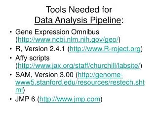
Tools Needed for Data Analysis Pipeline :. Gene Expression Omnibus ( http://www.ncbi.nlm.nih.gov/geo/ ) R, Version 2.4.1 ( http://www.R-roject.org ) Affy scripts ( http://www.jax.org/staff/churchill/labsite/ ) SAM, Version 3.00 ( http://genome-www5.stanford.edu/resources/restech.shtml )

E N D
Tools Needed for Data Analysis Pipeline: • Gene Expression Omnibus (http://www.ncbi.nlm.nih.gov/geo/) • R, Version 2.4.1 (http://www.R-roject.org) • Affy scripts (http://www.jax.org/staff/churchill/labsite/) • SAM, Version 3.00 (http://genome-www5.stanford.edu/resources/restech.shtml) • JMP 6 (http://www.jmp.com)
Annotated Affymetrix files (http://www.affymetrix.com/support/technical/annotationfilesmain.affx) • MeV, Version 4.0.01 (http://www.tm4.org) • Gene/Marker Batch Query Prototype (http://proto.informatics.jax.org/batchwi/index.do) • Ingenuity Pathways Analysis (www.ingenuity.com)
VLAD (http://proto.informatics.jax.org/pr) • MGI (http://www.informatics.jax.org/) • PubMed (http://www.ncbi.nlm.nih.gov/entrez/query.fcgi?DB=pubmed)
The first step is to locate data files at GEO: http://www.ncbi.nlm.nih.gov/geo/ Enter record # here
Are CEL (or raw) Data Files Available? • If Yes, continue to next slide. • If No, advance to slide # 70. GSE6077 will be used as an example
The next screen will indicate whether CEL files are available as supplementary files.
At the very bottom of the page you will see the link to download the raw data. Click on this.
You will then be prompted with a dialog box to download the files.
The files are downloaded as .gz files which then need to be unzipped
You’ll get a dialog box in which you can browse to the location you want the files saved. Ideally, you should have created a project folder ahead of time into which all data and analysis files will be kept. Then click OK.
You find them where you saved them. Put them in a folder like this. Your project folder should have an informative name, if possible, so you’ll know what’s in it later on.
Double click on the little boxes and they open as your .CEL files. These are the files that you’ll now perform Quality Control (QC) analysis on. Move the CEL Files out of the .gz folder (In this case put them in CEL_QC_instructions)
Move the .gz folder (which contains the compressed files) to another location, but don’t get rid of it. (I’m not sure why, but I found this was necessary in order to access the individual .CEL files) Ignore the Affy Scripts in this slide, there aren’t supposed to be there yet.
Next you’ll need three R scripts, in this order: AffyQC, Affyprocessing, and Affymaanova. Save them in your project folder along with R v2.4.1 (http://www.R-roject.org) and the .CEL files. http://www.jax.org/staff/churchill/labsite/ 2nd 3rd 1st
AffyQC • The AffyQC script will read in all CEL files in your working directory and perform Quality Control on them. • Visualizations of the quality of the data will be created and output as JPEG files. • Once the script is finished, you’ll find boxplot, histogram, and scatterplot JPEG files in your project folder as well as an RMA expression .DAT file.
Here is the affyQC script. The name for the workspace file should be changed to match the title of your project folder and/or data. Name of workspace file
Now fire up R and you’ll see a workspace console that looks like this. In the file menu, select Change Directory.
Browse to the same project folder where you have saved your .CEL files and the R scripts. Then click OK.
You’ll see a dialog box like this one. Only the affyQC and the affyprocessing scripts are saved as R files. The affymaanova script should be saved in notepad. (The reason for this will become apparent later on) This should not actually be in here.
When the QC script is done running, you’ll know because you’ll be back to the red > in the R Console.
Look in your project folder, and you’ll see these new files automatically downloaded and saved by the QC script.
Open up the rma.expr file in Excel and you’ll see the normalized expression values for each microarray sample (columns B through E). Column A contains the Probe ID.
I II III IV The Scatterplot .jpeg looks like this. In this case, the quality of the data looks pretty good. There is much less variation between biological replicates (quadrants II and IV) than between experimental conditions (quadrants I and III). For very large data sets sometimes the scatterplot doesn’t work. In these cases the rma.dat file can be opened in JMP and a scatterplot can be made there. See slide 100.
And the Boxplot .jpeg. The distribution in the four samples looks pretty consistent. No one sample looks way “out of line” with the others.
The next step is to run the affyprocessing script. What this script does is create a design file for the ANOVA analysis to follow. (It is possible to create the design file “by hand” as a text file and skip this step).
Some changes in the original script are necessary here as well (in the design matrix) so the names and numbers of samples fit the data. Note that for this example we have 4 samples – 2 Wild Type and 2 Mutant.
In the dialog box that pops up, this time select the affyprocessing script and click Open
When the affyprocessing script is done, you’ll know because you are back to the red > in the console window again. Look in your project folder and you should see the design file saved there now.
Open the design file with word pad, just to make sure it is correct. The first column (array) contains the CEL file names. The second file (strain) puts the samples into groups – in this case Wild Type vs. Mutant. The third column (sample) orders the samples. The fourth column (dye) labels all the samples with a “1”.
Now you are ready to run the maanova script. This is where things get a little more complicated …
Underlined in this script are the changes necessary to fit this particular data set. Log transformation is set at False, because the affyQC script does it.
More underlining of what might need to be changed to fit the particular data sets. This is the design file. This has been changed from 500 permutations to 1,000
And this is the end of the script. Name of workspace file
The final step is to run the affymaanova script. You’ll want to run this script line by line, just to make sure all the correct changes have been made. (It is more interactive this way) That’s why the script was saved as a text file rather than R source code.
Copy and paste the next line into the R console. (The lines preceded by a # are comment lines and they don’t get copied and pasted in)
Each time you see the red > you know that R is ready for the next command line.
Highlighted here is the real time consuming step in the program. Because we set it to run 1000 permutations instead of 500, it might take as long as an hour or so.
This is what your R Console should look like when you are all done with the affymaanova script.
Once again, you’ll see some new things automatically saved in the project folder you’ve been working in.
Here is the volcano plot. Looks very cool, but it isn’t necessary to spend lots of time staring at it.