Real-Time Control of Strike Point Motion in Fusion Tokamaks
Study on strike point control dynamics in fusion reactors; aim to design a PID controller keeping strike point centered. Testing with perturbations in PF1/PF2 requests.


Real-Time Control of Strike Point Motion in Fusion Tokamaks
E N D
Presentation Transcript
Office of Science Supported by Strike Point Control Dynamics College W&M Colorado Sch Mines Columbia U Comp-X General Atomics INEL Johns Hopkins U LANL LLNL Lodestar MIT Nova Photonics New York U Old Dominion U ORNL PPPL PSI Princeton U SNL Think Tank, Inc. UC Davis UC Irvine UCLA UCSD U Colorado U Maryland U Rochester U Washington U Wisconsin Culham Sci Ctr U St. Andrews York U Chubu U Fukui U Hiroshima U Hyogo U Kyoto U Kyushu U Kyushu Tokai U NIFS Niigata U U Tokyo JAEA Hebrew U Ioffe Inst RRC Kurchatov Inst TRINITI KBSI KAIST ENEA, Frascati CEA, Cadarache IPP, Jülich IPP, Garching ASCR, Czech Rep Egemen Kolemen,Princeton University in colloboration with D. Gates, C. Rowley, J. Kasdin, K. Taira NSTX 2009 Advanced Scenarios and Control
Motivation: Density Reduction via Strike Point Control • Density reduction depends on proximity of outer strike point to LLD-1 High d : ne reduced by 25% Low d : ne reduced by 50% LLD LLD Density Reduction R=0.65 R=0.84 R=0.84 R=0.65 Density Reduction 10cm 15cm 20cm 10cm 15cm 20cm Henry Kugel, R. Maingi, ORNL V. Soukhanovskii, LLNL Shown for different LLD-1 widths Shown for different LLD-1 widths
We expect the strike point predominantly depend on PF2L. • We can turn the system into a SISO black box control problem. • Introduce dynamics by assuming the plant as a time constant, , later. Preliminary Study: SISO System No Dynamics System PF2L=2 kAmp/MAmp PF2L=3 kAmp/MAmp PF2L=4 kAmp/MAmp • The change in the strike point with different PF2L current (isolver)
PF2L Scan: Shot 115495 • The change in the strike point for 115495.00501 with different PF2L current (isolver) • Change strike point location by changing PF2L while keeping the shape and PF1B, PF1AL, PF1AU, PF2U constant (let PF3L,PF5,PF3U vary to compensate). • While achieving (in order of importance): • Low Inner Gap, High Kappa • Scan by changing PF2L only:
PF2L Scan: Shot 120001 • The change in the strike point for 120001.00650 with different PF2L current (isolver) • Change strike point location by changing PF2L while keeping the shape and PF1B, PF1AL, PF1AU, PF2U constant (let PF3L,PF5,PF3U vary to compensate). • While achieving (in order of importance): • Low Inner Gap, High Kappa • Scan by changing PF2L only:
PF1B Scan: Shot 120001 • The change in the strike point for 120001.00650 with different PF1B current (isolver) • Change strike point location by changing PF2L while keeping the shape and PF1B, PF1AL, PF1AU, PF2U constant (let PF3L,PF5,PF3U vary to compensate). • While achieving (in order of importance): • Low Inner Gap, High Kappa • Scan by changing PF1B only:
Strike Point versus PF1B current For PF2L = 0.0047
Strike Point versus PF1B current For PF2L = 0.0057
PF1 versus PF2 For PF1B = 0.003 For PF2L = 0.0057 PF2L is 3-4 times more effective then PF1B in controlling the strike point
Aim: Design a Real Time Controller for the Strike Point Motion • Use the insight from the non-dynamic model to design a PID controller to keep the strike point at the center of LLD, with ~1 cm variation from the reference value. • Experiment: • Put perturbations in the PF1/PF2 requests & measure the strike point response. • Test and tune the strike point controller. • Study the compromise with respect to the loss in control for shape control and other control aims. • In this case, s=position and r=reference position of the strike point.
Experiment Procedure: Step Response and PID controller P PF1/2 • L = lag in time response • ΔCp (%) = the percentage change in output signal in response to the initial step disturbance • T = the time taken for this change to occur • N = ; where N is the reaction rate • R = • Then, for a given perturbation (P) Ziegler–Nichols PID controller
Experiment: Starting Condition Shot 115495.00501 is given as the requested profile. This is an old shot. Instead choose from shot 120001 with similar profile and same strike point.
Experiment Current Request: li Dependence • Depending on li and strike point distance choose the control input. • Experiment runs ~ 8-10 shots for PF2L and~ 8-10 shots for PF1B • Use shot120001 with strike point between 0 and 25 cm for PF2L and 0 and ~15 cm for PF1B. • Strike Point distance start with 0 then 25 cm (15 cm for PF1B) then interpolate as much points as possible in the experiment day. 0, 25, 12, 6, 18...(0 15 7 3 12 … for PF1B)
Extra dsf
Further Study: Multiple Control Input Variation Example x-point scan: Move it horizontally (Stefan Gerhardt) The following scan varies multiple variables at the same time. Try to keep the basic shape constant except for lower outer squareness.
Experiment Procedure: Step Response and Time Constant, . PF2L PF2L Choose two plasma shapes (and strike points) from the scan. Stabilize the plasma for the 1st shape. We know the coil currents need to take us to the 2nd equilibrium. Put a step input for the coil currents that gives the 2nd equilibrium. Measure the time constant of the strike point motion to the change in current. Repeat for many other equilibrium.
Aim: Design a Real Time Controller for the Strike Point Motion PID controller plant sensor • Use the insight from the non-dynamic model to design a PID controller to keep the strike point at the center of LLD, with ~1 cm variation from the reference value. • Experiment: • Put perturbations in the PF2 request & measure the response of the strike point. • Test and tune the strike point controller. • Study the compromise with respect to the loss in control for shape control and other control aims. • In this case, s=position and r=reference position of the strike point.
Aim: Design a Real Time Controller for the Strike Point Motion a
Aim: Design a Real Time Controller for the Strike Point Motion a
Used rtefit with no dynamics model to see the effect of the control PF coils on the strike point position. • Preliminary Study: • Strike point seems to be very much dependant on the X-point • It is not sensitive to the change in any coil but PF2L. Preliminary Study: No-Dynamics Model PF3L=1 kAmp Example Shot and the change of the strike point with different PF3L current. PF3L=2 kAmp PF3L=4 kAmp
Aim: Design a Real Time Controller for the Strike Point Motion a
Experiment Procedure • Choose two plasma shapes (and strike points) from the scan. • Stabilize the plasma for the 1st shape. • We know the coil currents need to take us to the 2nd equilibrium. • Put a step input for the coil currents that gives the 2nd equilibrium. • Measure the time constant of the strike point motion to the change in current. • Repeat for many other equilibrium.
Aim: Design a Real Time Controller for the Strike Point Motion PID controller plant sensor • Use the insight from the non-dynamic model to design a PID controller to keep the strike point at the center of LLD, with ~1 cm variation from the reference value. • Experiment (0.5 Day): • Put perturbations in the PF2 request & measure the response of the strike point. • Test and tune the strike point controller. • Study the compromise with respect to the loss in control for shape control and other control aims. • In this case, s=position and r=reference position of the strike point.
Aim: Design a Real Time Controller for the Strike Point Motion a
Liquid lithium divertor (LLD) on NSTX, enables experiments with the first complete liquid metal divertor target in a high-power device in 2009. • The location in the vacuum vessel is shown schematically in figure 1. • Reduced recycling with LLD. • The most important parameter that defines the density reduction is strike point position. Background: Liquid Lithium Divertor & Edge Density 1. Schematic of NSTX showing location of Liquid Lithium Divertor inside vacuum vessel 2. Edge density profiles calculating with UEDGE for NSTX Liquid Lithium Divertor assuming different recycling coefficients
A liquid lithium divertor (LLD) is being installed on NSTX, to enable experiments with the first complete liquid metal divertor target in a high-power device in 2009. The location in the vacuum vessel is shown schematically in Fig. 9. The LLD is a conic section with four 90-degree segments, each consisting of a 1.9 cm-thick copper plate with a 0.02 cm-thick stainless steel liner that is isolated toroidally with carbon tiles. Molybdenum will be plasma sprayed onto the liner in vacuum, to form a 0.01 cm-thick layer with 50% porosity. This will become the plasma-facing surface when filled with lithium, which will be kept liquid by resistive heaters in the plates. The present outer divertor (Fig. 1) consists of concentric rows of ATJ graphite tiles on copper baseplates. Lithium evaporated onto the tiles prior to a shot would solidify, and pump only while the hydrogenic atoms can react with the surface layer of the lithium coating. The LLD will replace part of these tiles with lithium that will be kept molten. Because the lithium will continue reacting with hydrogen or deuterium until it is volumetrically converted to hydrides,[12] the LLD is expected to provide better pumping than lithium coatings on carbon PFC’s. FIG. 9. Schematic of NSTX showing location of Liquid Lithium Divertor inside vacuum vessel Detailed edge plasma modeling has begun with the UEDGE transport code to simulate the effects of reduced recycling expected from the LLD.[13] The simulations start with adjusting the transport coefficients until the edge temperatures and densities match the data from the multipoint Thomson scattering diagnostic for existing NSTX plasmas. New profiles are then generated for a variety of recycling coefficients (Fig. 10). The results of the simulations have the same nonlinear radial dependence as the SOL measurements during high lithium evaporation. The simulations, however, do not show the linear density rise observed at the low lithium evaporation rate during NSTX experiments. This suggests that more work needs to be done on the transport modeling before further conclusions can be drawn from the UEDGE calculations. Background: Liquid Lithium Divertor & Edge Density Schematic of NSTX showing location of Liquid Lithium Divertor inside vacuum vessel FIG. 1. (left) Elevation of NSTX showing position of LITERs. (right) NSTX plan viewing indicating toroidal location of LITERs and coating regions blocked by center stack. FIG. 10. Edge density profiles calculating with UEDGE for NSTX Liquid Lithium Divertor assuming different recycling coefficients
LLD-1 Overview • Geometry:, 0.01cm thick, 50% porous Mo flame-sprayed on 0.02 cm SS brazed to 1.9 cm Cu. 20 cm wide, Ri = 0.65 m, Ro = 0.85 m. Li loading via LITER. • Operating temperature: typ. =205°C • Power Handling: SNL thermal analysis for the cases for the strike point on the LLD with peak Li temperature set at 400 °C, - can sustain a peak of ~2MW/m2 for 10s and 4 MW/m2 for ~3s. - Less Li, higher heat transfer. • Interlocks: similar to LITER (Heater Power off during fields, vacuum event, if temperature >set point,…..) - presently no automatic LLD-1 thermal interlock to interrupt plasma position or NBI - Fast and slow IR cameras will monitor LLD-1 front-face temperature. - Visible cameras will monitor divertor region. Li thermal conductivity is low. (~ W/m-°K 400 Cu, 150 Mo, 45 Li, 15 SS)
Day-1: Slowly increase Li and Test Pumping by LLD-1 on Outer Divertor to Provide Density Control for Inner Divertor Broad SOL Dα Profile, High δ Plasmas • Density reduction will depend on proximity of outer strike point to LLD-1 High d : reduce ne by 25% Soukhanovskii LLNL Density Reduction LLD 10cm 15cm 20cm R. Maingi, ORNL Shown for different LLD-1 widths
LLNL Day-2: Test Pumping by LLD-1 with Strike Point on Outer Divertor to Provide Density Control for Low δ Plasmas Low d : reduce ne by 50% Density Reduction LLD 10cm 15cm 20cm R=0.65 R=0.85 R. Maingi, ORNL Shown for different LLD-1 widths
Due to High Flux Expansion, Pumping by 20 cm Wide LLD-1 on Outer Divertor Will Provide Density Control for Both High and Low δ Plasmas • Density reduction will depend on proximity of outer strike point to LLD-1 High d : ne reduced by 25% Low d : ne reduced by 50% LLD LLD Density Reduction R=0.65 R=0.84 R=0.84 R=0.65 Density Reduction 10cm 15cm 20cm 10cm 15cm 20cm R. Maingi, ORNL V. Soukhanovskii, LLNL Shown for different LLD-1 widths Shown for different LLD-1 widths