Download
1 / 35
950 likes | 4.13k Vues
9. Fermi Surfaces and Metals. Construction of Fermi Surfaces Electron Orbits, Hole Orbits, and Open Orbits Calculation of Energy Bands Experimental Methods in Fermi Surface Studies. Fermi Surface : surface of ε = ε F in k -space. Separates filled & unfilled states at T = 0.

E N D
9. Fermi Surfaces and Metals • Construction of Fermi Surfaces • Electron Orbits, Hole Orbits, and Open Orbits • Calculation of Energy Bands • Experimental Methods in Fermi Surface Studies
Fermi Surface : surface of ε =εF in k-space Separates filled & unfilled states at T = 0. Close to a sphere in extended zone scheme. Looks horrible in reduced zone scheme. 2nd zone nearly half-filled
Reduced Zone Scheme Reduced Zone Scheme: k 1st BZ. k is outside 1st BZ. k= k + G is inside. Both & are lattice-periodic. So is → is a Bloch function
1-D Free Electrons / Empty Lattice Reduced zone scheme: εk is multi-valued function of k. Each branch of εk forms an energy band Bloch functions need band index: PWE
Periodic Zone Scheme εk single-valued εk multi-valued εnk single-valued εnk = εnk+G periodic E.g., s.c. lattice, TBA
Construction of Fermi Surfaces Zone boundary:
Harrison construction of free electron Fermi surfaces Points lying within at least n spheres are in the nth zone.
Nearly free electrons: Energy gaps near zone boundaries → Fermi surface edges “rounded”. Fermi surfaces & zone boundaries are always orthogonal.
Electron Orbits, Hole Orbits, and Open Orbits Electrons in static B field move on intersect of plane B &Fermi surface.
Nearly filled corners: P.Z.S. Simple cubic TBM P.Z.S.
Calculation of Energy Bands • Tight Binding Method for Energy Bands • Wigner-Seitz Method • Cohesive Energy • Pseudopotential Methods
Tight Binding Method for Energy Bands 2 neutral H atoms Ground state of H2 Excited state of H2 1s band of 20 H atoms ring.
TBM / LCAO approximation Good for valence bands, less so for conduction bands. α = s, p, d, … j runs over the basis atoms Bravais lattice , s-orbital only: ψk is a Bloch function since 1st order energy: Keep only on site & nearest neighbor terms:
For 2 H atoms ρ apart: Simple cubic lattice: 6 n.n. at Band width = 12 2 N orbitals in B.Z. = surface. 1 e per unit cell. periodic zone scheme
Fcc lattice: 12 n.n. at surface Band width = 24
Wigner-Seitz Method Bloch function: Schrodinger eq.: For k = 0, we have u0 is periodic in R l . is a Bloch function; can serve as an approximate solution of the Schrodinger eq. for k 0.
Prob 8 Wigner-Seitz B.C.: d /d r = 0 at cell boundaries. Wigner-Seitz result for 3s electrons in Na. Table 3.9, p.70 ionic r = 1.91A r0 of primitive cell = 2.08A n.n. r = 1.86A is constant over 7/8 vol of cell.
Cohesive Energy linear chain Na Table 6.1, p.139: F ~ 3.1 eV. K.E. ~ 0.6 F ~1.9 eV. • 5.15 eV for free atom. • 0 ~8.2 eV for u0 . • +2.7 eV for k at zone boundary. ~ 8.2+1.9 ~ 6.3 eV Cohesive energy ~ 5.15 +6.3 ~ 1.1 eV exp: 1.13 eV
Pseudopotential Methods Conduction electron ψ plane wave like except near core region. Reason: ψ must be orthogonal to core electron atomic-like wave functions. Pseudopotential: replace core with effective potential that gives true ψ outside core. Empty core model for Na (see Chap 10) Rc = 1.66 a0 . U ~ –50.4 ~ 200 Ups at r = 0.15 With Thomas-Fermi screening.
Typical reciprocal space Ups (see Chap 14) Empirical Pseudopotential Method Cohen
Experimental Methods in Fermi Surface Studies • Quantization of Orbits in a Magnetic Field • De Haas-van Alphen Effect • Extremal Orbits • Fermi Surface of Copper • Example: Fermi Surface of Gold • Magnetic Breakdown
Experimental methods for determining Fermi surfaces: • Magnetoresistance • Anomalous skin effect • Cyclotron resonance • Magneto-acoustic geometric effects • Shubnikov-de Haas effect • de Haas-van Alphen effect • Experimental methods for determining momentum distributions: • Positron annihilation • Compton scattering • Kohn effect Metal in uniform B field → 1/B periodicity
Quantization of Orbits in a Magnetic Field q = –e for electrons Bohr-Sommerfeld quantization rule: Phase corrector γ = ½ for free electrons B = const → Flux quantization Dirac flux quantum
→ For Δr B : Let A = Area in r-space, S = Area in k-space. → Hence Area of orbit in k-space is quantized If then Properties that depend on S are periodic functions of 1/B.
De Haas-van Alphen Effect dHvA effect: M of a pure metal at low T in strong B is a periodic function of 1/B. 2-D e-gas: PW in (B) dir. # of states in each Landau level = (spin neglected) See Landau & Lifshitz, “QM: Non-Rel Theory”, §112. Allowed levels B = 0 B 0
Number of e =48 D = 16 D = 19 D = 24 For the sake of clarity, n of the occupied states in the circle diagrams is 1 less than that in the level diagrams.
Critical field (No partially filled level at T = 0): s = highest completely filled level Black lines are plots of n = s ρ B, n = N = 50 at B = Bs. Red lines are plots of n = s N / ( N /ρ B ), n = N = 50 at N /ρ B = s .
Total energy in fully occupiedlevels: → for Total energy in partially occupied levels + 1: for for where
for where S = extremal area of Fermi surface B Section AA is extremal. Its contribution dominates due to phase cancellation effect.
Fermi Surface of Copper Cu / Au Monovalent fcc metal: n = 4 / a3 Shortest distance across BZ = distance between hexagonal faces Band gap at zone boundaries → band energy there lowered → necks Distance between square faces 12.57/a : necking not expected
Example: Fermi Surface of Gold dHvA in Au with B // [110]: Dogbone μ has period 210–9 gauss–1 for most directions → Table 6.1: → Period along [111] is 610–8 gauss–1 → → neck Dogbone area ~ 0.4 of belly area
Magnetic Breakdown → breakdown Change of connectivity ~ free electron-like Affected quantities ~ sensitive to connectivity : magnetoresistance E.g., hcp metals with zero (small if spin-orbit effect included) gap at hexagonal zone boundary Mg: Eg ~ 10–3 eV, εF ~ 10 eV, breakdown :