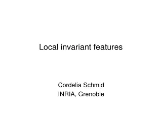
Local Invariant Features
Local Invariant Features. This is a compilation of slides by: Darya Frolova, Denis Simakov,The Weizmann Institute of Science Jiri Matas, Martin Urban Center for Machine Percpetion Prague Matthew Brown,David Lowe, University of British Columbia. Building a Panorama.


Local Invariant Features
E N D
Presentation Transcript
Local Invariant Features This is a compilation of slides by: Darya Frolova, Denis Simakov,The Weizmann Institute of Science Jiri Matas, Martin Urban Center for Machine Percpetion Prague Matthew Brown,David Lowe, University of British Columbia
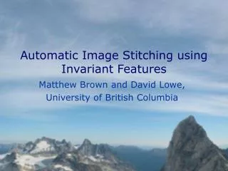
Building a Panorama M. Brown and D. G. Lowe. Recognising Panoramas. ICCV 2003
How do we build panorama? • We need to match (align) images
Matching with Features • Detect feature points in both images
Matching with Features • Detect feature points in both images • Find corresponding pairs
Matching with Features • Detect feature points in both images • Find corresponding pairs • Use these pairs to align images
Matching with Features • Problem 1: • Detect the same point independently in both images no chance to match! We need a repeatable detector
Matching with Features • Problem 2: • For each point correctly recognize the corresponding one ? We need a reliable and distinctive descriptor
More motivation… • Feature points are used also for: • Image alignment (homography, fundamental matrix) • 3D reconstruction • Motion tracking • Object recognition • Indexing and database retrieval • Robot navigation • … other
Selecting Good Features • What’s a “good feature”? • Satisfies brightness constancy • Has sufficient texture variation • Does not have too much texture variation • Corresponds to a “real” surface patch • Does not deform too much over time
Corner Detection: Introduction undistinguished patches: distinguished patches: “Corner” (“interest point”) detector detects points with distinguished neighbourhood(*) well suited for matching verification.
Detectors • Harris Corner Detector • Description • Analysis • Detectors • Rotation invariant • Scale invariant • Affine invariant • Descriptors • Rotation invariant • Scale invariant • Affine invariant
Harris Detector: Basic Idea “flat” region:no change in all directions “edge”:no change along the edge direction “corner”:significant change in all directions • We should easily recognize the point by looking through a small window • Shifting a window in anydirection should give a large change in intensity
Harris detector Based on the idea of auto-correlation Important difference in all directions => interest point
Corner Detection: Introduction + - > 0 Demo of a point + with well distinguished neighbourhood.
Corner Detection: Introduction + - > 0 Demo of a point + with well distinguished neighbourhood.
Corner Detection: Introduction + - > 0 Demo of a point + with well distinguished neighbourhood.
Corner Detection: Introduction + - > 0 Demo of a point + with well distinguished neighbourhood.
Corner Detection: Introduction + - > 0 Demo of a point + with well distinguished neighbourhood.
Corner Detection: Introduction + - > 0 Demo of a point + with well distinguished neighbourhood.
Corner Detection: Introduction + - > 0 Demo of a point + with well distinguished neighbourhood.
Corner Detection: Introduction + - > 0 Demo of a point + with well distinguished neighbourhood.
Harris detection • Auto-correlation matrix • captures the structure of the local neighborhood • measure based on eigenvalues of this matrix • 2 strong eigenvalues => interest point • 1 strong eigenvalue => contour • 0 eigenvalue => uniform region • Interest point detection • threshold on the eigenvalues • local maximum for localization
Harris detector Auto-correlation function for a point and a shift Discrete shifts can be avoided with the auto-correlation matrix
Harris detector Auto-correlation matrix
Window function Shifted intensity Intensity Window function w(x,y) = or 1 in window, 0 outside Gaussian Harris Detector: Mathematics Window-averaged change of intensity for the shift [u,v]:
Harris Detector: Mathematics Intensity change in shifting window: eigenvalue analysis 1, 2 – eigenvalues of M direction of the fastest change Ellipse E(u,v) = const direction of the slowest change (max)-1/2 (min)-1/2
Harris Detector: Mathematics Expanding E(u,v) in a 2nd order Taylor series expansion, we have,for small shifts [u,v], a bilinear approximation: where M is a 22 matrix computed from image derivatives:
Harris Detector: Mathematics 2 Classification of image points using eigenvalues of M: “Edge” 2 >> 1 “Corner”1 and 2 are large,1 ~ 2;E increases in all directions 1 and 2 are small;E is almost constant in all directions “Edge” 1 >> 2 “Flat” region 1
Harris Detector: Mathematics Measure of corner response: (k – empirical constant, k = 0.04-0.06)
Harris Detector: Mathematics 2 “Edge” “Corner” • R depends only on eigenvalues of M • R is large for a corner • R is negative with large magnitude for an edge • |R| is small for a flat region R < 0 R > 0 “Flat” “Edge” |R| small R < 0 1
Corner Detection: Basic principle distinguished patches: undistinguished patches: Image gradients ∇I(x,y) of undist. patches are (0,0) or have only one principle component. Image gradients ∇I(x,y) of dist. patcheshave two principle components. ⇒ rank ( ∑ ∇I(x,y)* ∇I(x,y) ⊤ ) = 2
Algorithm (R. Harris, 1988) 1. filter the image by gaussian (2x 1D convolution), sigma_d 2. compute the intensity gradients ∇I(x,y),(2x 1D conv.) 3. for each pixel and given neighbourhood, sigma_i: - compute auto-correlation matrix A = ∑∇I(x,y)* ∇I(x,y) ⊤ - and evaluate the response function R(A): R(A) >> 0 for rank(A)=2, R(A) → 0 for rank(A)<2 4. choose the best candidates (non-max suppression and thresholding)
Corner Detection: Algorithm (R. Harris, 1988) Harris response function R(A): R(A) = det (A) – k*trace 2(A) , [lamda1,lambda2] = eig(A)
Corner Detection: Algorithm (R. Harris, 1988) Algorithm properties: +“invariant” to 2D image shift and rotation + invariant to shift in illumination +“invariant” to small view point changes + low numerical complexity - not invariant to larger scale changes - not completely invariant to high contrast changes - not invariant to bigger view point changes
Corner Detection: Introduction Example of detected points
Corner Detection: Algorithm (R. Harris, 1988) Exp.: Harris points and view point change
Corner Detection:Harris points versus sigma_d and sigma_i ↑ Sigma_d Sigma_I →
Selecting Good Features l1 and l2 are large
Selecting Good Features large l1, small l2
Selecting Good Features small l1, small l2
Harris Detector • The Algorithm: • Find points with large corner response function R (R > threshold) • Take the points of local maxima of R
Harris Detector: Workflow Compute corner response R
Harris Detector: Workflow Find points with large corner response: R>threshold
Harris Detector: Workflow Take only the points of local maxima of R
Harris Detector: Summary • Average intensity change in direction [u,v] can be expressed as a bilinear form: • Describe a point in terms of eigenvalues of M:measure of corner response • A good (corner) point should have a large intensity change in all directions, i.e. R should be large positive
Corner Detection:Application 3D camera motion tracking / 3D reconstruction • Algorithm: • Corner detection • Tentative correspondences- by comparing similarity of the corner neighb. in the searching window (e.g. cross-correlation) • Camera motion geometry estimation (e.g. by RANSAC)- finds the motion geometry and consistent correspondences • 4. 3D reconstruction- triangulation, bundle adjustment
Contents • Harris Corner Detector • Description • Analysis • Detectors • Rotation invariant • Scale invariant • Affine invariant • Descriptors • Rotation invariant • Scale invariant • Affine invariant