Download
1 / 35
370 likes | 569 Vues
Statistical concepts of validation of microsimulation models. Philippe Finès Health Analysis Division Statistics Canada 24 November 2009. Introduction – renew. Validation is a process that includes steps in evaluation (ex: cost-effectiveness evaluation) assessment of uncertainty

E N D
Statistical concepts of validation of microsimulation models Philippe Finès Health Analysis Division Statistics Canada 24 November 2009
Introduction – renew • Validation is a process • that includes steps in • evaluation (ex: cost-effectiveness evaluation) • assessment of uncertainty • of which the outcome is a verdict • qualified by a criterion • “Valid” or “Not valid” • Green, Yellow, Red lights; • Score from 0 to 10 • based on statistical tests • inversely related to uncertainty? • and of which the purpose is to make recommendations
Related concepts • « Adjustment » • = steps done beforehand to make sure that simulation fits the data • Alignment • Calibration • Evaluation • = steps done to determine whether the program is adequate • Assessment • = steps done to analyse whether or not simulation fits reality • Assessment of uncertainty • Assessment of goodness of fit • Assessment of quality of reproduction of reality
Train of thought #1 • 1a: data observed in reality vs data generated in simulation • 1b: relationship in reality vs relationship in simulation
Train of thought #1 • Consider the relation (X,Y) • Reality: Phenomenon being observed • Y = f(X) + e • X has a « natural » variation se(X); and the « natural » variation of Y S(Y) depends on se(X) and e • If f, se(X), e are known, then for any value of X, Y and se(Y) are known
Train of thought #1 • Simulation: Phenomenon being created • X’= X + d(X) • Y’= Y + d(Y) • Y’= Y + d(X)= f(X) + d(Y)+ e • Y’ = f(X’- d(X)) + d(Y)+ e = f(X’) + e’ • If f, s(X’) and e are known, then for any value of X, Y’ and s(Y’) are known • But, we examine the following relation in the simulation: • Y’=g(X’)+e’ • How does the relation (X’,Y’) obtained in the simulation reproduces the relation (X,Y) observed in reality?
Train of thought #1 • One way to address this question is: • under which circumstances is this relationship (X’,Y’) close to relation (X,Y)? • Sufficient condition: d(X)=0, d(Y)=0. • This is achieved when simulated data reproduces « well » the reality (in the sense that simulated data can not be distinguished from the reality – this can be verified by a test) • Necessary condition: d(X) and d(Y) are « small » compared to e and to s(X). • In other words, the uncertainty of the simulation is « small » compared to the uncertainty of the model and the uncertainty of the data.
Validity =indistinguishability • A simulation model is « valid » if it presents indistinguishability • In the inputs X (i.e. if d(X) is not sign. different from 0) • In the outcomes X (i.e. if d(Y) is not sign. different from 0) • In the model (i.e. if e is not sig. diff. from 0) • This can be tested: include origin (simulation vs observed) as a dummy variable; test this variable
Statistical analysis to test null hypothesis – CI criterion • Rationale Using the approach of Haefner and Mankin et al (in Marks, 2007), we can examine the relationship between S (specific, historical output = reality), M (output of the model) and Q (the intersection of S and M)
Statistical analysis to test null hypothesis Model is complete and accurate (IDEAL CASE) Non null intersection between S and M model is useful, but incomplete and inaccurate No intersection between S and M model is useless Model is accurate but incomplete Model is complete but inaccurate
Statistical analysis to test null hypothesis – CI criterion • Estimation of the components of total uncertainty of results • Computation of the confidence intervals: • [Z-hat] (the C.I. for Z-hat) • [Zobs] (the C.I. for Zobs) • Comparison of confidence intervals: • [Z-hat] Í [Zobs] score = 100% (Best case) • ( [Z-hat] Ç [Zobs] ¹Æ and Z-hat Î [Zobs] and length ([Z-hat]) £ length ([Zobs]) ) or ( [Zobs] Ì [Z-hat] ) score = 80% • [Z-hat] Ç [Zobs] ¹Æ and Z-hat Î [Zobs] and length ([Z-hat]) > length ([Zobs]) score = 60% • [Z-hat] Ç [Zobs] ¹Æ and Z-hat Ï [Zobs] score = 40% • [Z-hat] Ç [Zobs] =Æ score = 0%
Statistical analysis to test null hypothesis – CI criterion • Possible cases (Assessment of a verdict):
Train of thought #2 • Uncertainties are larger in simulation, but by how much?
Train of thought #2 • In reality: X, Y • Uncertainty on X=s(X) • Uncertainty on the relationship (X,Y)=e • Uncertainty on Y=s(Y), which depends on s(X) and e • Elasticity of X with respect to Y = (delta(Y)/s(Y))/(delta(X)/s(X)), where delta(X) is defined as a function of s(X) (e.g. +/- 1.96*s(X)/sqrt(n))
Train of thought #2 • In the simulation: X’=X+d(X), Y’=Y+d(Y) • Uncertainty on X=s(X) • Uncertainty on the representation of X=d(X) • Uncertainty on X’=s(X’), which depends on s(X) and d(X) • Uncertainty on the relationship (X,Y)=e’ which depends on d(X), d(Y), e • Uncertainty on Y=s(Y), which depends on s(X) and e • Uncertainty on the representation of Y=d(Y) • Uncertainty on Y’=s(Y’), which depends on s(Y), d(Y) and e’ • Elasticity of X’ with respect to Y’ = (delta(Y’)/s(Y’))/(delta(X’)/s(X’)), where delta(X’) is defined as a function of s(X’) (e.g. +/- 1.96*s(X’)/sqrt(n)) • PRCC (Partial rank correlation coefficient) answers to questions such as how the output is affected if we increase (or decrease) a specific parameter cf. Marino et al, 2008: Simeone Marino, Ian B. Hogue, Christian J. Ray, Denise E. Kirschner. A methodology for performing global uncertainty and sensitivity analysis in systems biology, Journal of Theoretical Biology 254 (2008) 178– 196
Other notes • One could write variability of a result as the sum of uncertainty components • (cf. Marino et al, 2008: PRCC and eFAST) • PRCC (Partial rank correlation coefficient) answers to questions such as how the output is affected if we increase (or decrease) a specific parameter • eFAST (extended Fourier amplitude sensitivity test) indicate which parameter uncertainty has the greatest impact on output variability • (Our position:) A model would be considered valid if it does not add much variability compared to the one already present in the data • [(Xobs,Yobs)] [b-hat] [Z-hat]; [Z-hat] to be compared to [Zobs] • [Z-hat] (the C.I. for Z-hat) includes all the uncertainties implied in computation and simulation of Z-hat • [(Xobs,Yobs)]: variance estimates • [b-hat]: sensitivity analysis of parameters • Uncertainty due to model • Uncertainty due to simulation (=Monte-Carlo errors) • [Zobs] (the C.I. for Zobs) includes all the uncertainties implied in measure of Zobs • [Zobs]: variance estimates
Statistical analysis to test null hypothesis – Variance criterion • We consider that the model is valid if the following conditions are satisfied (the first 3 being essentially trivial): • In the training sample, E(ŷ) mY • In the test sample, E(ŷ) mY • Var (ŷ) in the training sample <= Var (y) in the test sample • In the test sample, Var (ŷ) <= Var (y), that is, the predicted values of the y are less dispersed than the original y values, even when using the coefficients obtained in the training sample. • We will repeat n times the technique of dividing the original sample into a training and a test samples (e.g. n=500). If the condition (iv) is realized at least 475 times (that is, 95% of the times), we conclude in this case that the model to predict y is valid.
Statistical analysis to test null hypothesis – MQE criterion • Mean Quadratic Error (MQE): • MQE = Variance + (Bias)2 where Variance is computed among the ŷi’s and Bias is the average gap between the ŷi’s and the yi’s • We want our model to be useful in the sense that • Biais² is much smaller than Variance • and MQE of the model is much smaller than Variance of the original yi’s (without any model). • MQE will be computed within the training sample and the test sample. Although we expect that MQE will be larger in the test sample than in the training sample, we will determine if it is not unreasonably larger than that of the training sample (say, not larger that 1.25 times MQE of the training sample). • We will repeat the splitting of the original sample in a test and a training sample, for B iterations (say, B=500). For each iteration, we will verify if the 3 conditions described above are satisfied a large number of times (say, 95%). • If it is not the case, then the model has to be questioned as his lack of stability will make the results in POHEM uneasy to interpret. • If it is the case, then we will say that the model is valid, and proceed to the validation of the parameters.
Train of thought #3 – Indistinguishability assessed in pivotal statistics
Train of thought #3 • To assess indistinguishability • One has to concentrate on pivotal statistics, i.e. the results for which the purpose is to validate the model. They represent “synthetic” results that are more easily interpretable and comparable between sources. • Ex: Z= number or proportion of deaths in a given year; Z= number or proportion of obese in a given year. • Some pivotal outcomes should include results after a certain amount of time. Ex: Z= number or proportion of deaths 20 years later; Z= number or proportion of obese 20 years later.
Train of thought #3 • For each node (ex: “Diabetes”), • we determine a pivotal statistics (ex: Prevalence in 10 years) • we determine the set of parameters that have an impact on the node • we examine the variability of the parameters • we build a series of scenarios that reproduce the variability of the parameters • we examine the impact of the scenarios on the range of the pivotal statistics
Train of thought #4 – conciliation of pivotal statistics and elasticity
Train of thought #4 • We also introduced the concept of « elasticity » of a statistics X as = the variation of Y / variation of X. • More precisely, elast(X,Y)=(delta Y/s(Y))/(delta X/s(X)), where delta X/s(X) is the « natural » variation of X.
Train of thought #4 • We want to introduce a theory that combines the concept of elasticity and of pivotal statistics. The problem is that it combines the Xs and the Ys. For simplicity, let us call X an input and Y and outcome. One tentative theory could be: • A pivotal statistics Y is an outcome such that for many inputs Xi, elast(Xi,Y) is « large » (i.e. the confidence interval widens significantly) • Ex: in POHEM-OA, LE and HALE are both related to incidence of OA, obesity, RR of obesity; but HALE varies relatively more than LE when incidence of OA, proportion of obese and RR of obesiy vary within their « natural » variation
Train of thought #4 • We have to limit ourselves to the pivotal statistics defined as the ones for which the elasticity is the largest: that means that we examine only the most sensitive outputs. • In other words, either we define pivotal statistics a priori (from the logical pathway) or we define them as the ones with precisely the largest elasticity.
Thank you! • Questions? • philippe.fines@statcan.gc.ca
Our position • In this presentation, we will only look at the uncertainty of the parameters, i.e. we perform sensitivity analysis.
Train of thought #2 • For each node, • we determine a pivotal statistics • that is easy to interpret • that can be compiled for real data • we determine the set of parameters that have an impact on the node • on either the main arc that leads to this node or all of them • we examine the variability of the parameters: • From a K-fold technique or from bootstrap technique, if they are available, we will get the distributions of the parameters • If k-fold and bootstrap techniques are not available, we will use standard error of the parameters • If this is not possible either, we will use only mean +/- 0.5*mean
Train of thought #2 • we build a series of scenarios that reproduce the variability of the parameters • using a “multi-way probabilistic” approach, we will implement the method suggested by Cronin et al. • The simulation will be run many times, with the values of the parameters randomly chosen from plausible combined distributions. The results will be presented as a distribution of model predictions. • This technique is a special case of Bayesian techniques where values of parameters are generated from an observed distribution. The challenge in this case will be to make sure that the plausible distributions mentioned are multidimensional: the values of the parameters will have to take into account the total and partial correlations between risk factors. • There will therefore be three methods: • No parameter uncertainty • Parametric bootstrap analysis • Cronin et al’s method
Train of thought #2 • we examine the impact of the scenarios on the range of the pivotal statistics • how much do the pivotal statistics vary? • Coefficient of sensitivity (CS) = elasticity = range of outcome / average of outcome • Is CS > or < 1? • We will conclude that if the results are “highly” sensitive to a group of parameters, it means that more emphasis has to be put on the accuracy of these parameters. • On the contrary, if they are relatively stable when the parameters vary within their permissible range, it means that the result is robust. • how much do the pivotal statistics stay close to the real data? • face validity • statistical analysis to test null hypothesis (H0) that “simulated results do not differ from real data” see next pages
Assessment of uncertainty • Uncertainty • According to Briggs, Sculpher, Buxton (for the context of HTA): • Uncertainty relating to variability in sample data • Uncertainty relating to the generalisability of results • Uncertainty relating to extrapolation • Uncertainty relating to analytical methods • Also (Wolf:) • uncertainty of random numbers (Cronin et al: stochastic variation) • parameter uncertainty • imputation error found in the starting-population data base • analyst’s ignorance about the true value of “unmeasured heterogeneity” • Also (Cronin et al:) • choice of the specified model structure
Assessment of uncertainty (Briggs, Sculpher, Buxton) • “The increased use of the clinical trial […], encourages greater use of formal statistical methods to handle some types of uncertainty systematically. • Sensitivity analysis is still1needed, however, […] in a number of contexts: • to deal with uncertainty in relation to data inputs for which no clear sample exists; • to attempt to increase the generalisability of the study; • to handle uncertainty associated with attempts to extrapolate away from the primary data source, in order to make the results more comprehensive [also in Weinstein, 2006] • to explore the implications of selecting a particular analytical method from amongst alternatives when no widely accepted approach exists” (p. 101) • Therefore, Briggs, Sculpher, Buxton oppose statistical methods to sensitivity analysis. However, they are not incompatible. (1): Emphasis ours
Assessment of uncertainty (Briggs, Sculpher, Buxton) • Sensitivity analyses • Simple sensitivity analysis • One-way • Multi-way • Threshold analysis • Identify the critical value of parameter (s) above or below which the conclusion of a study will change • Analysis of extremes • High cost: combination of all pessimistic assumptions about costs • Low cost: combination of all optimistic assumptions about costs • Probabilistic sensitivity analysis • Taking into account the distribution of values
Assessment of uncertainty (Briggs, Sculpher, Buxton) • Uncertainty • Uncertainty relating to variability in sample data • Uncertainty relating to the generalisability of results • Uncertainty relating to extrapolation • Uncertainty relating to analytical methods • Sensitivity analyses • Simple sensitivity analysis • Threshold analysis • Analysis of extremes • Probabilistic sensitivity analysis
Assessment of uncertainty – bootstrap approach (Cronin et al) Sensitivity analysis on the parameters • No parameter uncertainty • Parametric bootstrap analysis • Parameter sampling design • (Latin square design)