Download
1 / 10
100 likes | 210 Vues
Learn about different types of Evolution Strategies like Simple (1+1)-ES, (μ+1)-ES, (μ+λ)-ES, and (μ,λ)-ES with detailed procedures, similarities, and applications. Understand implementation, attributes, and success rules of ES.

E N D
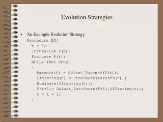
Evolution Strategies • An Example Evolution Strategy Procedure ES{ t = 0; Initialize P(t); Evaluate P(t); While (Not Done) { Parents(t) = Select_Parents(P(t)); Offspring(t) = Procreate(Parents(t)); Evaluate(Offspring(t)); P(t+1)= Select_Survivors(P(t),Offspring(t)); t = t + 1; }
Evolution Strategies • There are basically 4 types of ESs • The Simple (1+1)-ES • The (+1)-ES (The first multimembered ES) • The (+)-ES, and • The (,)-ES.
Evolution Strategies:The Simple (1+1)-ES • The simple (1+1)-ES has the following attributes: • Individuals are represented as follows: • <xi,0,xi,1,…, xi,n-1,i>, where n is the number of variables • Offspring are created as follows: +i,j = k,j * exp(0 * N(0,1)); x+i,j = xk,j + +i,jN+i,j(0,1); Where j represents the jth variable. And where 0 1/sqrt(n)(Global Learning Rate) • Uses the 1/5 Success Rule to Adapt the Step Size: • If more than 1/5th of the mutations cause an improvement (in the objective function) then multiply by 1.2, • If less than 1/5th of the mutations cause an improvement, then multiply by 0.8.
Evolution Strategies:The Simple (1+1)-ES • Procedure simpleES{ t = 0; Initialize P(t); /* = 1, = 1 */ Evaluate P(t); while (t <= (4000-)/){ for (i=0; i<1; i++){ Create_Offspring(<xi,yi,i>,<x+i,y+i,+i>): +i = i * exp(0 * N(0,1)); x+i = xi + +iN+i,x(0,1); y+i = yi + +iN+i,y(0,1); fit+i = Evaluate(<x+i,y+i>); } P(t+1) = Better of 2 individuals; t = t + 1; } }
Evolution Strategies:The Simple (1+1)-ES • How is a simple (1+1)-ES similar to a (1+1)-Standard EP? • In what ways are the two different?
Evolution Strategies:The (+1)-ES • Since the (+1)-ES is multi-membered, crossover can be used. • According to, Bäck, T., Hoffmeister, F, and Schwefel, H.-P. (1991). “A Survey of Evolution Strategies”, The Proceedings of the 4th International Conference on Genetic Algorithms, R. K. Belew and L. B. Booker Eds., pp. 2-9, Morgan Kaufmann. [can be found at: http://citeseer.nj.nec.com/back91survey.html] • Uniform Crossover (also referred to a discrete recombination) can be used on the variable values as well as the strategy parameter. • Adaptation of the step-size is not used in the (+1)-ES.
Evolution Strategies: The (+1)-ES Procedure (+1)-ES{ t = 0; Initialize P(t); /* of individuals */ Evaluate P(t); while (t <= (4000-)){ Create_Offspring(<xi,yi,i>,<x+i,y+i,+i>): +i = i * exp(0 * N(0,1)); x+i = xi + +iN+i,x(0,1); y+i = yi + +iN+i,y(0,1); fit+i = Evaluate(<x+i,y+i>); P(t+1) = Best of the +1 individuals; t = t + 1; } }
Evolution Strategies:The (+)-ES • In the (+)-ES, an individual, i, is represented as follows: • <xi,0,xi,1,…, xi,n-1,i,0,i,1,…,i,n-1>, where n is the number of variables • Offspring are created by as follows: • +i,j = k,j * exp(’* N(0,1) + * N+i(0,1)); x+i,j = xk,j + +i,jN+i,j(0,1); • Where j represents the jth variable, • ’ 1/sqrt(2n) /* Global Learning Rate */ • 1/sqrt(2*sqrt(n)) /* Individual Learning Rate */ • The 1/5th success rule is used.
Evolution Strategies:The (+)-ES Procedure (+)-ES{ t = 0; Initialize P(t); /* of individuals */ Evaluate P(t); while (t <= (4000-)/){ for (i=0; i<; i++){ Create_Offspring(<xk,yk,k,x,k,y>, <x+i,y+i,+i,x,+i,y>): +i,x = k,x * exp(’* N(0,1) + * N+i(0,1)); x+i = xi + +i,x N+i,x(0,1); +i,y = k,y * exp(’* N(0,1) + * N+i(0,1)); y+i = yi + +i,y N+i,y(0,1); fit+i = Evaluate(<x+i,y+i>); } P(t+1) = Best of the + individuals; t = t + 1; } }
Evolution Strategies:The (,)-ES Procedure (,)-ES{ t = 0; Initialize P(t); /* of individuals */ Evaluate P(t); while (t <= (4000-)/){ for (i=0; i<; i++){ Create_Offspring(<xk,yk,k,x,k,y>, <x+i,y+i,+i,x,+i,y>): +i,x = k,x * exp(’* N(0,1) + * N+i(0,1)); x+i = xi + +i,x N +i,x(0,1); +i,y = k,y * exp(’* N(0,1) + * N+i(0,1)); y+i = yi + +i,y N +i,y(0,1); fit+i = Evaluate(<x+i,y+i>); } P(t+1) = Best of the offspring; t = t + 1; } }