The Production Process
The Production Process. Production Analysis. Production Function Q = f(K,L) Describes available technology and feasible means of converting inputs into maximum level of output, assuming efficient utilization of inputs:

The Production Process
E N D
Presentation Transcript
Production Analysis • Production Function Q = f(K,L) • Describes available technology and feasible means of converting inputs into maximum level of output, assuming efficient utilization of inputs: • ensure firm operates on production function (incentives for workers to put max effort) • use cost minimizing input mix • Short-Run vs. Long-Run Decisions • Fixed vs. Variable Inputs
Total Product • Cobb-Douglas Production Function • Example: Q = f(K,L) = K.5 L.5 • K is fixed at 16 units. • Short run production function: Q = (16).5 L.5 = 4 L.5 • Production when 100 units of labor are used? Q = 4 (100).5 = 4(10) = 40 units
Marginal Product of Labor • Continuous case: MPL = dQ/dL • Discrete case: arc MPL = DQ/DL • Measures the output produced by the last worker. • Slope of the production function
Average Product of Labor • APL = Q/L • Measures the output of an “average” worker. • Slope of the line from origin onto the production function
Three significant points are: Max MPL(TP inflects) Max APL = MPL MPL = 0(Max TP) A line from the origin is tangent to Total Product curve at the maximum average product. Law of Diminishing Returns (MPs) TP increases at an increasing rate (MP > 0 and ) until inflection , continues to increase at a diminishing rate (MP > 0 but ) until max and then decreases (MP < 0). Increasing MP Diminishing MP Negative MP
Isoquant • The combinations of inputs (K, L) that yield the producer the same level of output. • The shape of an isoquant reflects the ease with which a producer can substitute among inputs while maintaining the same level of output. • Slope or Marginal Rate of Technical Substitution can be derived using total differential of Q=f(K,L) set equal to zero (no change in Q along an isoquant)
Cobb-Douglas Production Function • Q = KaLb • Inputs are not perfectly substitutable (slope changes along the isoquant) • Diminishing MRTS: slope becomes flatter • Most production processes have isoquants of this shape • Output requires both inputs K-K1 || -K2 Q3 Increasing Output Q2 Q1 L1 < L2 L
K Increasing Output Q2 Q3 Q1 L Linear Production Function • Q = aK + bL • Capital and labor are perfect substitutes (slope of isoquant is constant)y = ax + bK = Q/a - (b/a)L • Output can be produced using only one input
Q3 K Q2 Q1 Increasing Output Leontief Production Function • Q = min{aK, bL} • Capital and labor are perfect complements and cannot be substituted (no MRTS <=> no slope) • Capital and labor are used in fixed-proportions • Both inputs needed to produce output
Isocost K New Isocost for an increase in thebudget (total cost). • The combinations of inputs that cost the same amount of moneyC = K*PK + L*PL • For given input prices, isocosts farther from the origin are associated with higher costs. • Changes in input prices change the slope (Market Rate of Substitution) of the isocost lineK = C/PK - (PL/PK)L C0 C1 L K New Isocost for a decrease in the wage (labor price). L
-PL/PK < -MPL/MPKMPK/PK< MPL/PL K Point of Cost Minimization-PL/PK = -MPL/MPKMPK/PK= MPL/PL -PL/PK > -MPL/MPKMPK/PK> MPL/PL Q L Long Run Cost Minimization Min cost where isocost is tangent to isoquant (slopes are the same) Expressed differently: MP (benefit) per dollar spent (cost) must be equal for all inputs
Returns to Scale Return (MP): How TP changes when one input increases RTS: How TP changes when all inputs increase by the same multiple > 0 Q = f(K, L) Q = 50K½L½Q = 100,000 + 500L + 100KQ = 0.01K3 + 4K2L + L2K + 0.0001L3