Regression Analysis Assumptions and Techniques
Explore the key assumptions, techniques, and challenges in regression analysis, including multicollinearity, dummy variables, autocorrelation, non-linear relationships, heteroskedasticity, and outliers.

Regression Analysis Assumptions and Techniques
E N D
Presentation Transcript
The regression model has both constants (, b) and variables (X, Y) • The “fit” of the regression equation to the data is numerically expressed by the r2 statistic. • The b for each indep var can be tested for statistical significance using a t test. • The overall model is tested for statistical significance using the F ratio.
Assumptions of the regression model • Like all statistics, the regression model has a number of underlying assumptions. • T-test assumes a t distribution • z scores assumes data is normally distributed • We will discuss some of the more common ones.
Multicollinearity • When 2 or more independent variables in the model are highly correlated with one another. • Result: bias in the partial regression coefficients • Test: by correlating each variable with the others • Fix: drop all but one of highly correlated variables or combine into a single variable
“Dummy” variables • Regression analysis assumes the use of continuous, interval level data • Two types • dichotomous variables (two possible states) • polychotomous variables • may be nominal or ordinal
Dummy variables • Dichotomous variable • male/female; Republican/Democrat • yes/no • Essentially, a case has or does not have a particular characteristic • Example: last week’s regression model predicting entry GS grade • field of education • veterans’ preference • minority female
Polychotomous variables - a number of possible states • often, sometimes, rarely, never • region of country (South, Midwest, East, West) • When using exclude one of the categories • Include three 0/1 variables; eliminate one category • the excluded variable becomes the reference category
Autocorrelation • A nonrandom relationship among a variable’s values at different time periods • consistent patterns such as seasonal data • Often found in time series data
Autocorrelation • Result: biased t-ratios, confidence limits, and hypotheses tests • Test: plot the residuals - look for distinctive patterns • Fix: introduce another independent variable that explains some of the unexplained variance • more commonly: use a statistical model other than OLS
Nonlinear relationships • OLS assumes a linear relationship (remember the straight line we drew based on the regression equation?) • Some of out data does not provide a linear relationship • economic data • population data • data with built-in growth factor
Nonlinear relationships • We test for this using a scatterplot. • Does the relationship appear linear? • Fix: transform one of the variables
Heteroskedasticity • When the effect of X on Y is not equal across all ranges of Y • Result: affects size of standard error, thus biasing hypothesis test results.
Outliers • Extreme values • when a particular (or number of them) don’t seem to fit in with the other data. • Problem: can bias the regression parameters

