Download
1 / 52
620 likes | 931 Vues
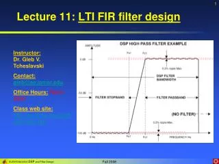
Lecture 11: LTI FIR filter design. Instructor: Dr. Gleb V. Tcheslavski Contact: gleb@ee.lamar.edu Office Hours: Room 2030 Class web site: http://ee.lamar.edu/gleb/dsp/index.htm. Preliminary considerations. FIR filter:. (11.2.1). transfer function.

E N D
Lecture 11: LTI FIR filter design Instructor: Dr. Gleb V. Tcheslavski Contact:gleb@ee.lamar.edu Office Hours: Room 2030 Class web site:http://ee.lamar.edu/gleb/dsp/index.htm
Preliminary considerations FIR filter: (11.2.1) transfer function unit-pulse response BTW, using our “rational notation”: (11.2.2) Here M-1 is the filter order. M is the number of filter’s coefficients. Assuming that M is odd: (11.2.3)
Preliminary considerations For an FIR filter to have a linear phase: (11.3.1) That means an even symmetry of the coefficients. (11.3.2) Remember: FIR filters are always stable (no poles other than at the origin)!
Preliminary considerations Since the filter is stable: (11.4.1) As a result of symmetry: Here is a real function of frequency. (11.4.2)
We can use to design ANY amplitude of frequency response: LPF, HPF, BPF,… When changes sign, the phase undergoes an abrupt change of 1800 Preliminary considerations Therefore: (11.5.1) Generalized linear phase In M is even: (11.5.2)
Preliminary considerations An FIR filter will also have a linear phase in the case of odd symmetry of filter coefficients (antisymmetric impulse response), i.e.: (11.6.1) It can be shown that (11.6.2) (11.6.3) Therefore: (11.6.4) (11.6.5) BTW: (11.6.6)
Preliminary considerations Thus: (11.7.1) Generalized linear phase Summarizing, a unit-pulse response of a GLP FIR filter must satisfy: (11.7.2) (11.7.3) (11.7.4) We only need to specify (M-1)/2 (odd M) or M/2 unique coefficients (even M).
Preliminary considerations Combining (11.7.2) and (11.7.3), we arrive at: (11.8.1) Example: if M = 5: Has two pairs of reciprocal zeros. firls(4,[0 0.25],[1 0]);
Preliminary considerations There are four types of real GLP FIR filters: Type I: symmetric hn, odd M(number of coefficients) – even order. Type II: symmetric hn, even M Type III: antisymmetric hn, odd M Type IV: antisymmetric hn, even M indicate “structural zeros”
Preliminary considerations 1. For M = 4, symmetrical pulse response ( Type II FIR): (11.10.1) 2. For M = 4, antisymmetrical pulse response ( Type IV FIR): This is where structural zeros come from… (11.10.2) 3. For M = 5, antisymmetrical pulse response ( Type III FIR): (11.10.3)
Preliminary considerations As a result of structural zeros… Type II FIR HPF would have a zero at - specs will be violated! Type III FIR HPF would have a zero at - specs will be violated! Type IV FIR LPF would have a zero at 0 - specs will be violated! If something like tis happens, increase or decrease the FIR order to change the type of your filter. We need to be careful with selection of filter orders!
1. Least-square error minimization The desired magnitude response (something we specify): (11.12.1) Filter coefficients could be found as: (11.12.2) Example: Ideal LPF (11.12.3) Not causal, infinite length! We need to preserve the main features while making the filter causal.
1. Least-square error minimization The filter specified by (11.12.3) has an infinite impulse response. Therefore, we need to truncate it at some point to make an FIR filter. As a criterion for such truncation, we need to minimize the approximation error (the difference between the desired and the truncated frequency responses). Therefore, the objective is to find a finite-duration impulse response sequence, whose DTFT would approximate the desired frequency response. The magnitude of the frequency response of the “truncated filter”: (11.13.1) Where L and U are points at which the pulse response was truncated. We need to minimize the least-square integral error of approximation.
1. Least-square error minimization In particular: (11.14.1) (11.14.2) Apparently, to minimize R (LS error), we select ht,n = hd,nfor n = L…U. Moreover, GLP requires symmetry of filter coefficients, therefore L = -U. The best finite length approximation of the ideal infinite length impulse response in the LS error sense is obtained by truncation. To make the resulting FIR causal, we need to shift it by L radians.
1. Least-square error minimization Relating the point of truncation to the FIR filter order: L = (M – 1)/2 (11.15.1) Note: filter length M (number of filter coefficients) can be both even or odd. Non-causal Causal
2. Windowing effects We can view the truncation of the infinite impulse response of an ideal filter as windowing. In frequency domain, this operation is equivalent to convolution of a frequency response of the window function with the frequency response of an ideal filter. (11.16.1) from the Modulation theorem: (11.16.2) W R: Gibbs phenomenon (comes from truncated Fourier series) Ripples of equal magnitude in PB and SB Transition band – another window artifact
2. Windowing effects: window types As discussed previously, different window functions can be used… Fixed windows: Window properties Filter properties
2. Windowing effects: window types Rectangular: (11.18.1) Hanning: (11.18.2) (11.18.3) Hamming: Blackman: (11.18.4)
2. Windowing effects: window types Adjustable windows: Kaiser window: (11.19.1) Where: (11.19.2) Normally, 15-20 terms in the summation are sufficient. Note: if = 0, WnK = WnR.
2. Windowing effects: window types Properties: Hanning Hamming Blackman Kaiser window is the most frequently used for the FIR filter design.
2. Windowing: experimental design For the given transition band: (11.21.1) Stop-band attenuation: (11.21.2) Order estimate: (11.21.3) Adjustable parameter: (11.21.4) M controls transition band, changes ripples. Note: in practice, ripples in SB and PB are approximately equal. If this does not hold, need to select minimum of s, p.
2. Windowing: experimental design Example 11.1: design an FIR LPF using a Kaiser window for the following specs: The transition band: Order: Parameter: We select M = 24, = 4. The filter is given by (11.15.1) with the cutoff frequency: The transfer function: The resulting filter is a type II FIR which is ok for LPF.
3. Frequency sampling The desired frequency response (11.23.1) can be specified by its frequency samples at equally spaced (discrete) frequencies: (11.23.2) Where (11.23.3) = 0.5: = 0: 2/M 2/M /M (11.23.4)
3. Frequency sampling The sampled frequency response will be: (11.24.1) Evaluating IDFT: (11.24.2) Therefore, we can compute the filter coefficients from the specified M frequency samples. Since hn is real: (11.24.3) Since hn is symmetric, we only need to specify either (M+1)/2 (M is odd) or M/2 (M is even) frequency samples to determine the pulse response.
3. Frequency sampling We can rewrite the FIR filter frequency response (11.7.4) as: (11.25.1) Sampled at the frequencies (11.25.2) the response becomes: (11.25.3)
3. Frequency sampling Here: (11.26.1) For simplicity, we specify the following set of real frequency samples: (11.26.2) Therefore: (11.26.3)
3. Frequency sampling Case 1: (11.27.1) (11.27.2)
3. Frequency sampling (11.28.1) Since hn is real: (11.28.2) (11.28.3) Since Hr is real: (11.28.4)
3. Frequency sampling Therefore: (11.29.1) The number of coefficients (frequency samples) to be specified: (11.29.2) - forced zero at z = -1 Since the unit-pulse response is already evaluated, we can estimate the corresponding frequency response as its zero-padded DFT: and check whether the specifications are satisfied.
3. Frequency sampling Case 2: The desired frequency samples: (11.30.1) (11.30.2) (11.30.3)
3. Frequency sampling Case 3: The desired frequency samples: (11.31.1) (11.31.2) (11.31.3)
3. Frequency sampling Case 4: The desired frequency samples: (11.32.1) (11.32.2) (11.32.3)
3. Frequency sampling We specify the desired response in the SB and the PB only… The stopband attenuation in this case (only SB and PB samples are given) is approximately -20 dB. Alternatively, we can add transition sample(s) and make the frequency response smoother. The stopband attenuation would be: for one TB sample: approximately -40 dB. for two TB sample: approximately -60 dB. for three TB sample: approximately -80 dB.
3. Frequency sampling The transition band sample(s) “optimized” experimentally are: Effects of adding TB sample(s) are increased SB attenuation and wider TB. These samples must be optimized for the situation. Selection of the offset can help too. Note: we can specify any desired frequency response at the samples but not in between! Ultimately, we can view all frequency samples as the TB samples, which leads to an optimal (equiripple) design.
4. Optimal equiripple design We are interested in a LP filter satisfying the following requirements: (11.35.1) Considering four FIR types: Type 1: symmetric pulse response, odd M. (11.35.2) The real-valued frequency response: (11.35.3) (11.35.4)
4. Optimal equiripple design Type 2: symmetric pulse response, even M. (11.36.1) The real-valued frequency response: (11.36.2) (11.36.3) Or: (11.36.4) Where: (11.36.5)
4. Optimal equiripple design Type 3: antisymmetric pulse response, odd M. (11.37.1) The real-valued frequency response: (11.37.2) (11.37.3) Or: (11.37.4) Where: (11.37.5)
4. Optimal equiripple design Type 4: antisymmetric pulse response, even M. (11.38.1) The real-valued frequency response: (11.38.2) (11.38.3) Or: (11.38.4) Where: (11.38.5)
4. Optimal equiripple design Therefore, we can express the frequency response for all FIR types as: (11.39.1) (11.39.2) Where:
4. Optimal equiripple design The desired frequency response: (11.40.1) We can compute and compare it to . Adjusting P() and selecting filter type, we can obtain the desired frequency characteristic. We introduce the weighting function on the approximation error: (11.40.2) If s < p – bigger error in the passband is allowed.
4. Optimal equiripple design The weighted approximation error: (11.41.1) Where the modified weighting function and the modified desired frequency response are: (11.41.2) (11.41.3)
4. Optimal equiripple design For the given error function E(e j), the Chebyshev (mini-max) approximation problem is to determine the filter parameters k that minimize the maximum absolute error over the frequency bands of interest: (11.42.1) Usually, the frequency bands of interest are specified as: (11.42.2) a disjoint union of the passband and the stopband: 0 - p and s - (for a LPF). That is we “ignore” the transition band. More precisely speaking, error over the TB will not be optimized. The solution of this problem can be found via the alternation theorem.
4. Optimal equiripple design The alternation theorem A necessary and sufficient conditions for to be unique and best approximation to in S is that the error function E(ej) exhibit at least L + 2 extremal frequencies in S. That is, there must exist at least L + 2 frequencies {i}, such that: (11.43.1) (11.43.2) (11.43.3) I.e., error alternates in sign between two successive extremal frequencies.
4. Optimal equiripple design: Example Example 11.2: design a LPF. Since both the desired frequency response Hdr and the weighting function W are piecewise constants: (11.44.1) Consequently, the frequencies {i} that correspond to the peaks of the error function E(e j) also correspond to the peaks of Hr(e j), i.e., where the frequency response meets the specified error tolerance. Since Hr(e j) is a polynomial of degree L: (11.44.2) Hr(e j) has at most L-1 local minima and maxima and, therefore, at most L+1 extremal frequencies (bandages) since we add = 0 and = . Furthermore, the band-edge frequencies p and s are also extrema of the error function. Therefore, E(e j) has at most L+3 extremal frequencies.
4. Optimal equiripple design: Example However, from the alternation theorem, there are at least L+2 extremal frequencies in E(e j).Thus the error function for the LPF design will have either L+2 or L+3 (extra ripple filters) extremal frequencies. At the specified extremal frequencies n: alternations (11.45.1) Here represents the maximum value of the error function E(e j). (11.45.2) or alternatively: (11.45.3)
4. Optimal equiripple design: Example We can consider the {k} and as the unknown (to be determined) design parameters for the given extremal frequencies. Therefore: (11.46.1) • Note: initially, both the design parameters and the extremal frequencies are unknown. The above system can be solved by the iterative algorithm (Remez exchange algorithm): • Guess the set of L + 1 extremal frequencies; • Solve for {k} and ; • Determine the error function as in (11.39.1); • Determine the new set of L + 1 extremal frequencies and go to 2)… • Keep running until E(e j) - convergence.
4. Optimal equiripple design Alternatively, we can compute analytically [Rabiner ‘75]: (11.47.1) (11.47.2) where: Therefore, the initial guess of the L + 2 extremal frequencies allows us to compute the maximum value of the error . Thus: (11.47.3)
4. Optimal equiripple design Since we know that the polynomial at the points xn = cos nhas the values: (11.48.1) the Lagrange interpolation formula can be used, which leads to (11.48.2) (11.48.3) Here: (11.48.4) (11.48.5)
4. Optimal equiripple design Having the solution for P, we can compute the error function: (11.49.1) on a dense set of frequency points. Usually, 16M frequency points are sufficient. If the error exceeds the estimated tolerance , we select a new set of frequencies corresponding to the L+2 largest peaks of error function and the procedure starts from (11.45.1). New set of critical frequencies will lead to increased . As a result, the algorithm produces the optimal solution with equal ripples in the PB and the SB for the given M. The order of the filter can be estimated as: (11.49.2)
Summary Historically, the window-based algorithm was the first proposed method for FIR design. Its major disadvantage is the lack of precise control of the critical frequencies, such as s and p. These values, in general, depend on the type of the window and the filter length M. The frequency sampling method is attractive since it specifies an arbitrary frequency response at the uniformly spaced frequencies and the transition band is a multiple of 2/M. However, no control for the response in between the samples. The Chebyshev approximation method provides a total control of the filter specifications and may lead to an equiripple design. This way, the approximation error is spread evenly across the PB and SB, which leads to an optimal filter. This method is usually preferred.


![[f´‚nE˘RIks]](https://cdn0.slideserve.com/636013/f-ne-riks-dt.jpg)