Download
1 / 35
360 likes | 592 Vues
LECTURE 5 Topic 1: Metabolic network and stoichiometric matrix Topic 2: Hierarchical clustering of multivariate data. Typical network of metabolic pathways. Reactions are catalyzed by enzymes. One enzyme molecule usually catalyzes thousands reactions per second (~ 10 2 -10 7 )

E N D
LECTURE 5Topic 1: Metabolic network and stoichiometric matrixTopic 2: Hierarchical clustering of multivariate data
Typical network of metabolic pathways Reactions are catalyzed by enzymes. One enzyme molecule usually catalyzes thousands reactions per second (~102-107) The pathway map may be considered as a static model of metabolism
What is a stoichiometric matrix? For a metabolic network consisting of m substances and r reactions the system dynamics is described by systems equations. The stoichiometric coefficients nij assigned to the substance Si and the reaction vj can be combined into the so called stoichiometric matrix.
Example reaction system and corresponding stoichiometric matrix There are 6 metabolites and 8 reactions in this example system stoichiometric matrix
Binary form of N To determine the elementary topological properties, Stiochiometric matrix is also represented as a binary form using the following transformation nij’=0 if nij =0 nij’=1 if nij ≠0
Stiochiometric matrix is a sparse matrix Source: Systems biology by Bernhard O. Palsson
Information contained in the stiochiometric matrix Stiochiometric matrix contains many information e.g. about the structure of metabolic network , possible set of steady state fluxes, unbranched reaction pathways etc. • 2 simple information: • The number of non-zero entries in column i gives the number of compounds that participate in reaction i. • The number of non-zero entries in row j gives the number of reactions in which metabolite j participates. So from the stoicheometric matrix connectivities of all the metabolites can be computed
Information contained in the stiochiometric matrix There are relatively few metabolites (24 or so) that are highly connected while most of the metabolites participates in only 2 reactions
Information contained in the stiochiometric matrix In steady state we know that The right equality sign denotes a linear equation system for determining the rates v This equation has non trivial solution only for Rank N < r(the number of reactions) K is called kernel matrix if it satisfies NK=0 The kernel matrix K is not unique
Information contained in the stiochiometric matrix The kernel matrix K of the stoichiometric matrix N that satisfies NK=0, contains (r- Rank N) basis vectors as columns Every possible set of steady state fluxes can be expressed as a linear combination of the columns of K
Information contained in the stiochiometric matrix - And for steady state flux it holds that J = α1 .k1 + α2.k2 With α1= 1 and α2 = 1, , i.e. at steady state v1 =2, v2 =-1 and v3 =-1 That is v2 and v3 must be in opposite direction for the steady state corresponding to this kernel matrix which can be easily realized.
Information contained in the stiochiometric matrix Reaction System Stoicheometric Matrix The stoicheomatric matrix comprises r=8 reactions and Rank =5 and thus the kernel matrix has 3 linearly independent columns. A possible solution is as follows:
Information contained in the stiochiometric matrix Reaction System The entries in the last row of the kernel matrix is always zero. Hence in steady state the rate of reaction v8 must vanish.
Information contained in the stiochiometric matrix If all basis vectors contain the same entries for a set of rows, this indicate an unbranched reaction path Reaction System The entries for v3 , v4 and v5 are equal for each column of the kernel matrix, therefore reaction v3 , v4 and v5 constitute an unbranched pathway . In steady state they must have equal rates
Elementary flux modes and extreme pathways The definition of the term pathway in a metabolic network is not straightforward. A descriptive definition of a pathway is a set of subsequent reactions that are in each case linked by common metabolites Fluxmodes are possible direct routes from one external metabolite to another external metabolite. A flux mode is an elementary flux mode if it uses a minimal set of reactions and cannot be further decomposed.
Elementary flux modes and extreme pathways Extreme pathway is a concept similar to elementary flux mode The extreme pathways are a subset of elementary flux modes The difference between the two definitions is the representation of exchange fluxes. If the exchange fluxes are all irreversible the extreme pathways and elementary modes are equivalent If the exchange fluxes are all reversible there are more elementary flux modes than extreme pathways One study reported that in human blood cell there are 55 extreme pathways but 6180 elementary flux modes
Elementary flux modes and extreme pathways Source: Systems biology by Bernhard O Palsson
Elementary flux modes and extreme pathways Elementary flux modes and extreme pathways can be used to understand the range of metabolic pathways in a network, to test a set of enzymes for production of a desired product and to detect non redundant pathways, to reconstruct metabolism from annotated genome sequences and analyze the effect of enzyme deficiency, to reduce drug effects and to identify drug targets etc.
AtpB AtpA AtpG AtpE AtpA AtpH AtpB AtpH AtpG AtpH AtpE AtpH In many cases for example in case of microarray gene expression analysis the data is multivariate type. An Introduction to Bioinformatics Algorithms by Jones & Pevzner Hierarchical Clustering Data is not always available as binary relations as in the case of protein-protein interactions where we can directly apply network clustering algorithms.
Hierarchical Clustering We can convert multivariate data into networks and can apply network clustering algorithm about which we will discuss in some later class. If dimension of multivariate data is 3 or less we can cluster them by plotting directly. An Introduction to Bioinformatics Algorithms by Jones & Pevzner
Hierarchical Clustering Some data reveal good cluster structure when plotted but some data do not. Data plotted in 2 dimensions However, when dimension is more than 3, we can apply hierarchical clustering to multivariate data. In hierarchical clustering the data are not partitioned into a particular cluster in a single step. Instead, a series of partitions takes place.
Hierarchical Clustering Hierarchical clustering is a technique that organizes elements into a tree. A tree is a graph that has no cycle. A tree with n nodes can have maximum n-1 edges. A Graph A tree
Hierarchical Clustering • Hierarchical Clustering is subdivided into 2 types • agglomerative methods, which proceed by series of fusions of the n objects into groups, • and divisive methods, which separate n objects successively into finer groupings. • Agglomerative techniques are more commonly used Data can be viewed as a single cluster containing all objects to n clusters each containing a single object .
Hierarchical Clustering Distance measurements Euclidean distance between g1 and g2
Hierarchical Clustering An Introduction to Bioinformatics Algorithms by Jones & Pevzner In stead of Euclidean distance correlation can also be used as a distance measurement. For biological analysis involving genes and proteins, nucleotide and or amino acid sequence similarity can also be used as distance between objects
Hierarchical Clustering • An agglomerative hierarchical clustering procedure produces a series of partitions of the data, Pn, Pn-1, ....... , P1. The first Pn consists of n single object 'clusters', the last P1, consists of single group containing all n cases. • At each particular stage the method joins together the two clusters which are closest together (most similar). (At the first stage, of course, this amounts to joining together the two objects that are closest together, since at the initial stage each cluster has one object.)
Hierarchical Clustering An Introduction to Bioinformatics Algorithms by Jones & Pevzner Differences between methods arise because of the different ways of defining distance (or similarity) between clusters.
Hierarchical Clustering How can we measure distances between clusters? Single linkage clustering Distance between two clusters A and B, D(A,B) is computed asD(A,B)= Min { d(i,j) : Where object i is in cluster A and object j is cluster B}
Hierarchical Clustering Complete linkage clustering Distance between two clusters A and B, D(A,B) is computed asD(A,B)= Max { d(i,j) : Where object i is in cluster A and object j is cluster B}
Hierarchical Clustering Average linkage clustering Distance between two clusters A and B, D(A,B) is computed asD(A,B) = TAB / ( NA * NB) Where TAB is the sum of all pair wise distances between objects of cluster A and cluster B. NAand NB are the sizes of the clusters A and B respectively. Total NA * NBedges
Hierarchical Clustering Average group linkage clustering Distance between two clusters A and B, D(A,B) is computed asD(A,B) = = Average { d(i,j) : Where observations i and j are in cluster t, the cluster formed by merging clusters A and B } Total n(n-1)/2 edges
Hierarchical Clustering Alizadeh et al. Nature 403: 503-511 (2000).