Understanding Digital Filters: Fundamentals and Applications
Explore box filters and lowpass filters, learn about frequency response, impulse response, edge detection, and derivative calculations in digital signal processing.


Understanding Digital Filters: Fundamentals and Applications
E N D
Presentation Transcript
What have we seen so far? • So far we have seen… • Box filter • Moving average filter • Example of a lowpass • passes low frequencies • small, gradual changes in the signal are passed • higher frequencies are attenuated (reduced/removed/suppressed)
Applied by cross correlation (sum of products) of image f and mask h If mask is centered about origin, (x,y) in image: If origin, (x,y), in image is aligned with (0,0) in mask:
But how do we know what the application of an arbitrary mask actually does to the image?
For simplicity, let us just consider 1D signals (e.g., mono audio)
Our moving average (box) filter Example of a lowpass filter (passes low frequencies, attenuates high frequencies) y[n] = 1/3 x[n-1] + 1/3 x[n] + 1/3 x[n+1] More generally y[n] = h[-1] x[n-1] + h[0] x[n] + h[1] x[n+1]
Lowpass filters Input: (before) x(t) = 0.5*sin(t) + sin(3*t+pi/3) + sin(5*t+pi/8) Output: (after) y(t) = 0.5*sin(t) + sin(3*t+pi/3)
So how can we determine how our moving average filter behaves? • 11 point and 51 point moving average filters (on the previous slide) obviously produce different outputs even when given the same input! • Answer: By determining how a particular filter responds to an impulse (their impulse response function).
So given …,h[-1],h[0],h[1],… how can we plot the impulse reponse. • Perform the z-transform (the discrete version of the Laplace transform) of h resulting H. • Plot H on the unit circle. The magnitude of H (abs(H) or |H|) is amplitude and the angle of H (arg(H)) is the phase. • Say we have a 3 point box filter: h[-1]=h[0]=h[1]=1/3.
So given …,h[-1],h[0],h[1],… how can we plot the impulse response. • Say we have an 11 point box filter: h[-5]=h[-4]=h[-3] =h[-3] =h[-2] =h[-1] =h[0] =h[1] =h[2] =h[3] =h[4] =h[5]=1/11.
Frequency response (dB) and phase of 3 and 11 point box filters.
Spectral inversion:How to make a highpass filter the easy way. • Change the sign of each sample in the filter kernel. • Add 1 to the sample at the center of symmetry. • highpass lowpass • lowpass highpass • bandpass bandreject (stopband) • bandreject bandpass
Bandreject (stopband) = lowpass + highpass (lowpass or highpass)
Application of filters Edge detection
Recall the first derivative test from calculus: Let the function f be continuous on some interval (c-,c+) containing the critical point c. • If f’(x)>0 for x in (c-,c) and f’(x)<0 for x in (c,c+), then f has a local maximum at c. • If f’(x)<0 for x in (c-,c) and f’(x)>0 for x in (c,c+), then f has a local minimum at c.
Can we calculate the first derivative of an image? Let h1=[-1, 1]. Then f’(x) = g(x) = f(x)h1(x) where is cross correlation. So we can then search f’(x) for extrema where: • 0 occurs • -a,+b occurs • +a,-b occurs
Recall the following from calculus regarding the second derivative: Let f be continuous on [a,b] and at least twice differentiable on (a,b). If f’’(x)>0 on (a,b), then f is concave up on [a,b], while if f’’(x)<0 on (a,b), then f is concave down on [a,b].
Recall the second derivative test from calculus: Let the function f be defined on an open interval containing the critical point c where f’(c)=0, and let f’’ be continuous on this interval. • If f’’(c)<0, then c is a local maximum point. • If f’’(c)>0, then c is a local minimum point. • If f’’(c)=0, then no conclusion is possible without further investigation.
Also recall: A point c is called an inflection point of f if: • f is continuous at c; • the graph of f has a tangent line (possibly vertical) at [c,f(c)]; • f is concave up on one side of c and concave down on the other side.
We can consider the inflection point to be the location of an edge!
Can we calculate the second derivative of an image? Let h1=[-1, 1]. Then f’(x) = f(x)h1(x) Then f’’(x) = f’(x)h1(x) • where is cross correlation. So we can then search f’’(x) for edges where: • 0 occurs • -a,+b occurs • +a,-b occurs
Can we calculate the second derivative of an image? A better way … let h2=[1, -2, 1]. Then f’’(x) = f(x)h2(x) Much more computationally efficient. Where does h2 come from? From [-1, 1] [1, -1] which is h1 * h1 where * is convolution.
Applying masks to images Convolution: Discrete form:
Frequency response (dB) and phase of first derivative filter.
Frequency response (dB) of first and second derivative filters.