Chapter 3: Maximum-Likelihood and Bayesian Parameter Estimation (part 2)

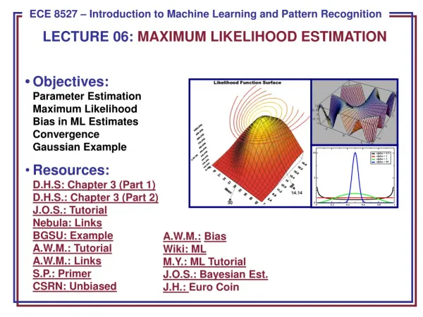
2. Chapter 3:Maximum-Likelihood and Bayesian Parameter Estimation (part 2) • Bayesian Estimation (BE) • Bayesian Parameter Estimation: Gaussian Case • Bayesian Parameter Estimation: General Estimation • Problems of Dimensionality • Computational Complexity • Component Analysis and Discriminants • Hidden Markov Models

3. Bayesian Estimation (Bayesian learning to pattern classification problems) • In MLE  was supposed fix • In BE  is a random variable • The computation of posterior probabilities P(i | x) lies at the heart of Bayesian classification • Goal: compute P(i | x, D) Given the sample D, Bayes formula can be written Pattern Classification, Chapter 1 3

4. To demonstrate the preceding equation, use: Pattern Classification, Chapter 1 3

5. Bayesian Parameter Estimation: Gaussian Case Goal: Estimate  using the a-posteriori density P( | D) • The univariate case: P( | D)  is the only unknown parameter (0 and 0 are known!) Pattern Classification, Chapter 1 4

6. Reproducing density Identifying (1) and (2) yields: Pattern Classification, Chapter 1 4

7. Pattern Classification, Chapter 1 4

8. The univariate case P(x | D) • P( | D) computed • P(x | D) remains to be computed! It provides: (Desired class-conditional density P(x | Dj, j)) Therefore: P(x | Dj, j) together with P(j) And using Bayes formula, we obtain the Bayesian classification rule: Pattern Classification, Chapter 1 4

9. Bayesian Parameter Estimation: General Theory • P(x | D) computation can be applied to any situation in which the unknown density can be parametrized: the basic assumptions are: • The form of P(x | ) is assumed known, but the value of  is not known exactly • Our knowledge about  is assumed to be contained in a known prior density P() • The rest of our knowledge  is contained in a set D of n random variables x1, x2, …, xn that follows P(x) Pattern Classification, Chapter 1 5

10. The basic problem is: “Compute the posterior density P( | D)” then “Derive P(x | D)” Using Bayes formula, we have: And by independence assumption: Pattern Classification, Chapter 1 5

11. Problems of Dimensionality • Problems involving 50 or 100 features (binary valued) • Classification accuracy depends upon the dimensionality and the amount of training data • Case of two classes multivariate normal with the same covariance Pattern Classification, Chapter 1 7

12. If features are independent then: • Most useful features are the ones for which the difference between the means is large relative to the standard deviation • It has frequently been observed in practice that, beyond a certain point, the inclusion of additional features leads to worse rather than better performance: we have the wrong model ! Pattern Classification, Chapter 1 7

13. 7 7 Pattern Classification, Chapter 1 7

14. Computational Complexity • Our design methodology is affected by the computational difficulty • “big oh” notation f(x) = O(h(x)) “big oh of h(x)” If: (An upper bound on f(x) grows no worse than h(x) for sufficiently large x!) f(x) = 2+3x+4x2 g(x) = x2 f(x) = O(x2) Pattern Classification, Chapter 1 7

15. “big oh” is not unique! f(x) = O(x2); f(x) = O(x3); f(x) = O(x4) • “big theta” notation f(x) = (h(x)) If: f(x) = (x2) but f(x)  (x3) Pattern Classification, Chapter 1 7

16. Complexity of the ML Estimation • Gaussian priors in d dimensions classifier with n training samples for each of c classes • For each category, we have to compute the discriminant function Total = O(d2..n) Total for c classes = O(cd2.n)  O(d2.n) • Cost increase when d and n are large! Pattern Classification, Chapter 1 7

17. Component Analysis and Discriminants • Combine features in order to reduce the dimension of the feature space • Linear combinations are simple to compute and tractable • Project high dimensional data onto a lower dimensional space • Two classical approaches for finding “optimal” linear transformation • PCA (Principal Component Analysis) “Projection that best represents the data in a least- square sense” • MDA (Multiple Discriminant Analysis) “Projection that best separatesthe data in a least-squares sense” Pattern Classification, Chapter 1 8

18. Hidden Markov Models: • Markov Chains • Goal: make a sequence of decisions • Processes that unfold in time, states at time t are influenced by a state at time t-1 • Applications: speech recognition, gesture recognition, parts of speech tagging and DNA sequencing, • Any temporal process without memory T = {(1), (2), (3), …, (T)} sequence of states We might have 6 = {1, 4, 2, 2, 1, 4} • The system can revisit a state at different steps and not every state need to be visited Pattern Classification, Chapter 1 10

19. First-order Markov models • Our productions of any sequence is described by the transition probabilities P(j(t + 1) | i (t)) = aij Pattern Classification, Chapter 1 10

20. Pattern Classification, Chapter 1 10

21.  = (aij, T) P(T |) = a14 . a42 . a22 . a21 . a14 . P((1) = i) Example: speech recognition “production of spoken words” Production of the word: “pattern” represented by phonemes /p/ /a/ /tt/ /er/ /n/ // ( // = silent state) Transitions from /p/ to /a/, /a/ to /tt/, /tt/ to er/, /er/ to /n/ and /n/ to a silent state Pattern Classification, Chapter 1 10