Download
1 / 28
280 likes | 306 Vues
ASV Chapter s. 1 - Sample Spaces and Probabilities 2 - Conditional Probability and Independence 3 - Random Variables 4 - Approximations of the Binomial Distribution 5 - Transforms and Transformations 6 - Joint Distribution of Random Variables 7 - Sums and Symmetry

E N D
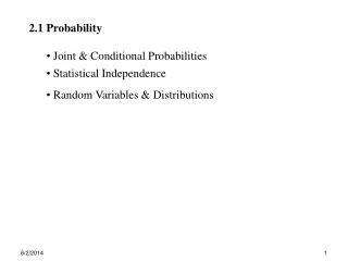
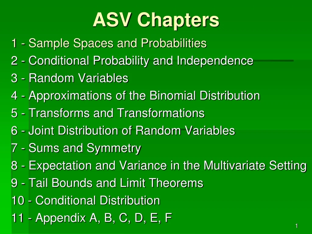
ASV Chapters 1 - Sample Spaces and Probabilities 2 - Conditional Probability and Independence 3 - Random Variables 4 - Approximations of the Binomial Distribution 5 - Transforms and Transformations 6 - Joint Distribution of Random Variables 7 - Sums and Symmetry 8 - Expectation and Variance in the Multivariate Setting 9 - Tail Bounds and Limit Theorems 10 - Conditional Distribution 11 - Appendix A, B, C, D, E, F
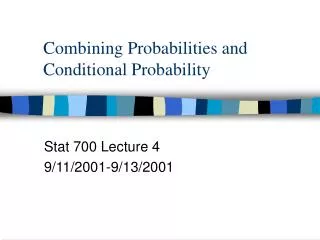
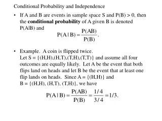
Population Distribution of X Suppose X ~ N(μ, σ), then… X = Age of women in U.S. at first birth Each of these individual ages xis a particular value of the random variableX. Most are in the neighborhood of μ, but there are occasional outliers in the tails of the distribution. Density x4 x1 x5 x2 x3 … etc…. σ = 1.5 X x x x x x μ= 25.4
Population Distribution of X Suppose X ~ N(μ, σ), then… Sample, n = 400 Sample, n = 400 Sample, n = 400 Sample, n = 400 Sample, n = 400 X = Age of women in U.S. at first birth Density How are these values distributed? … etc…. Each of these sample mean values is a “point estimate” of the population mean μ… σ = 1.5 X μ= 25.4
Population Distribution of X Suppose X ~ N(μ, σ), then… Suppose X ~ N(μ, σ), then… for any sample size n. “standard error” X = Age of women in U.S. at first birth Sampling Distribution of The vast majority of sample meansare extremely close to μ, i.e., extremely small variability. Density Density How are these values distributed? … etc…. Each of these sample mean values is a “point estimate” of the population mean μ… σ = 1.5 X μ= 25.4 μ= μ=
Population Distribution of X Suppose X ~ N(μ, σ), then… Suppose X ~ N(μ, σ), then… for any sample size n. for large sample size n. “standard error” X = Age of women in U.S. at first birth Suppose X ~ N(μ, σ), then… Sampling Distribution of The vast majority of sample meansare extremely close to μ, i.e., extremely small variability. Density Density … etc…. Each of these sample mean values is a “point estimate” of the population mean μ… σ = 2.4 X μ= 25.4 μ= μ=
Population Distribution of X X ~ Anything with finite μ and σ Suppose XN(μ, σ), then… for any sample size n. for large sample size n. “standard error” X = Age of women in U.S. at first birth Suppose X ~ N(μ, σ), then… Sampling Distribution of The vast majority of sample meansare extremely close to μ, i.e., extremely small variability. Density Density … etc…. Each of these sample mean values is a “point estimate” of the population mean μ… σ = 2.4 X μ= 25.4 μ= μ=
Density “standard error” Density
Probability that a single house selected at random costs less than $300K = ? = Cumulative area under density curve for X up to 300. = Z-score Density Example: X = Cost of new house ($K) “standard error” Density 300
Probability that a single house selected at random costs less than $300K = ? 0.6554 = Z-score Density Example: X = Cost of new house ($K) “standard error” Density 300
Probability that a single house selected at random costs less than $300K = ? 0.6554 = Z-score • Probability that the sample mean of n = 36 houses selected at random is less than $300K = ? = Cumulative area under density curve for up to 300. Density Example: X = Cost of new house ($K) “standard error” Density $12.5K 300 300
Probability that a single house selected at random costs less than $300K = ? 0.6554 = Z-score • Probability that the sample mean of n = 36 houses selected at random is less than $300K = ? 0.9918 = Z-score Density Example: X = Cost of new house ($K) “standard error” Density $12.5K 300 300
large approximately “standard error” Density Density mild skew
large ~ CENTRAL LIMIT THEOREM ~ continuous or discrete, approximately as n , “standard error” Density Density
large ~ CENTRAL LIMIT THEOREM ~ continuous or discrete, approximately as n , Example: X = Cost of new house ($K) “standard error” Density Density
Probability that a single house selected at random costs less than $300K = ? = Cumulative area under density curve for X up to 300. • Probability that the sample mean of n = 36 houses selected at random is less than $300K = ? 0.9918 = Z-score Example: X = Cost of new house ($K) “standard error” Density Density $12.5K 300 300
possibly log-normal… but remember Cauchy and 1/x2, both of which had nonexistent … CLT may not work! More on CLT… heavily skewed tail each based on 1000 samples
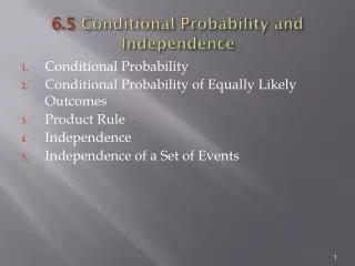
Population Distribution of X X ~ Dist(μ, σ) Random Variable More on CLT… X = Age of women in U.S. at first birth If this first individual has been randomly chosen, and the value of X measured, then the result is a fixed number x1, with no random variability… and likewise for x2, x3, etc. DATA! Density BUT… X
Population Distribution of X X ~ Dist(μ, σ) Random Variable More… X = Age of women in U.S. at first birth If this first individual has been randomly chosen, and the value of X measured, then the result is a fixed number x1, with no random variability… and likewise for x2, x3, etc. DATA! Density However, if this is not the case, then this first “value” of X is unknown, thus can be considered as a random variable X1 itself… and likewise for X2, X3, etc. BUT… X The collection {X1, X2, X3, …, Xn} of “independent, identically-distributed” (i.i.d.) random variables is said to be a random sample.
Population Distribution of X X ~ Dist(μ, σ) Random Variable Sample, size n More… X = Age of women in U.S. at first birth CENTRAL LIMIT THEOREM Sampling Distribution of etc…… Density Claim: for anyn Proof: Density X
Population Distribution of X X ~ Dist(μ, σ) Random Variable More… X = Age of women in U.S. at first birth CENTRAL LIMIT THEOREM Sampling Distribution of etc…… Density Claim: for anyn Proof: Density X
continuous discrete More on CLT… Recall… Normal Approximation to the Binomial Distribution Suppose a certain outcome exists in a population, with constant probability. We will randomly select a random sample of n individuals, so that the binary “Success vs. Failure” outcome of any individual is independent of the binary outcome of any other individual, i.e., nBernoulli trials (e.g., coin tosses). P(Success) = P(Failure) = 1 – Then X is said to follow a Binomial distribution, written X ~ Bin(n, ), with “probability function” p(x) = , x = 0, 1, 2, …, n. Discrete random variable X = # Successes (0, 1, 2,…, n) in a random sample of size n
continuous discrete Normal Approximation to the Binomial Distribution Suppose a certain outcome exists in a population, with constant probability. We will randomly select a random sample of n individuals, so that the binary “Success vs. Failure” outcome of any individual is independent of the binary outcome of any other individual, i.e., nBernoulli trials (e.g., coin tosses). P(Success) = P(Failure) = 1 – CLT See Prob 5.3/7 Then X is said to follow a Binomial distribution, written X ~ Bin(n, ), with “probability function” p(x) = , x = 0, 1, 2, …, n. Discrete random variable X = # Successes (0, 1, 2,…, n) in a random sample of size n
continuous discrete ?? Normal Approximation to the Binomial Distribution Suppose a certain outcome exists in a population, with constant probability. We will randomly select a random sample of n individuals, so that the binary “Success vs. Failure” outcome of any individual is independent of the binary outcome of any other individual, i.e., nBernoulli trials (e.g., coin tosses). P(Success) = P(Failure) = 1 – CLT Then X is said to follow a Binomial distribution, written X ~ Bin(n, ), with “probability function” p(x) = , x = 0, 1, 2, …, n. Discrete random variable X = # Successes (0, 1, 2,…, n) in a random sample of size n