Quantitative EDX Analysis in TEM Practical Development, Limitations and Standards
210 likes | 531 Vues
Quantitative EDX Analysis in TEM Practical Development, Limitations and Standards. F. Nieto Dto. de Mineralog ía y Petrología Instituto Ándaluz de Ciencias de la Tierra Universidad de Granada-CSIC.

Quantitative EDX Analysis in TEM Practical Development, Limitations and Standards
E N D
Presentation Transcript
Quantitative EDX Analysis in TEM Practical Development, Limitations and Standards F. Nieto Dto. de Mineralogía y Petrología Instituto Ándaluz de Ciencias de la Tierra Universidad de Granada-CSIC
the concentration of an element (Ce) in a sample generates a specific, characteristic X-ray intensity • if a standard of known composition (Cst) is taken for element e, we can measure the intensity ratio Ie/Ist Ce / Cst = K Ie / Ist where Ie is the intensity measured in the sample and Ist is the intensity measured in the standard K is a correction factor that includes three different effects: • atomic number (Z) • X-ray absorption by the sample (A) • X-ray fluorescence by the sample (F) • The complete correction procedure is termed ZAF Correction and it is complex, requiring a computer forcalculation.
If the analysis is performed on a thin sample that is transparent to the electrons, then the correction procedure is considerably simplified. • Factors A and F can be minimized and consequently ignored the volume analyzed is reduced, so that the spatial resolution is much greater • The ZAF correction is • neither necessary • nor possible • This is both • the simplification and • the limitation of TEM microanalysis it is difficult to determine the sample thickness at a particular point
The analytical quality is not equal to that obtained with SEM or EMPA (error for TEM are around 10% to 15%, lower detection limit is about 0.3% wt) Since the sample is thin (50-100 nm), the analyzed area is the same as the excited area, that is, equal to the spot size. It is therefore possible to perform microanalyses as small as the electron beam size In accordance with the above factors, there are clearly delimited, although complementary, fields of use for these techniques (SEM or EPMA vs AEM) Although EDX detectors and transmission electron microscopes (TEMs) equipped with the STEM were developed in 1960, it was not until 1975 that Cliff and Lorimer demonstrated the possibility of doing the afore-mentioned simplification This step revolutionized the microanalysis of thin samples This technique is known as AEM (Analytical Electron Microscopy)
Method of Cliff and Lorimer (1975) This approximation is based on the assumption that, in thin samples, there is no absorption or fluorescence effect (thin foil criterion) the ratio of the X-ray intensities of two elements, A and B, is proportional to the ratio of concentrations: CA / CB = KAB (IA / IB) KAB = K factor of A with respect to B • These factors can be calculated • theoretically • the commercial programs for the equipment include theoretical factors • experimentally • with standards The curve relating Z with KAB is characteristic for every electron microscope, every accelerating voltage and every detector.
The calculation is simple, not requiring a computer, and the background subtraction process is much simpler than for SEM or EPMA since there is less background in thin samples. The K factors are not radically different than 1 (except for light elements), which allows a qualitative determination of minerals based on the peak height since it gives a simple, direct spectrum interpretation.
CA / CSi KASi (IA / ISi) = CB / CSi KBSi (IA / ISi) • Since most of the minerals analyzed in geology are silicates, the factors are usually expressed in relation to Si. • Non-silicate compounds can still be analyzed, of course, but it is slightly more complex. Therefore KAB = KASi / KBSi
Microanalysis by EDX with TEM is a relative method in which the results are the atomic proportions between the elements present. • CA/CB can be determined, but not CA and CB. • This basic limitation of the method is not a serious problem in mineralogy or similar fields, since the calculation of formulas is always done with normalizations to a known factor such as • the proportions of a given element • total number of positive or negative charges • total cations • etc.
Relative proportions • To be normalized according to some criterium • Cations = 2 • Si = 1 • +charges = 6 It is apyroxene! Si O3 ( Mg, Ca,Fe) Si O3 Mg0.4 Ca0.4 Fe0.2 The results are correctly expressed by the formulas
Ways to express the KAB factors as a function of the units of concentration. Definition of factors. A concentration can be expressed in different ways: • weight percentage of the element (CA) • weight percentage of the oxide (C´A) • atomic concentration of the element -number of atoms- (NA) To transform from one type of concentration to another, we use the molecular weight of the oxide and the number of atoms in the oxide formula, or the atomic weight of the element. The equation of Cliff and Lorimer depends on the concentration expression used, resulting in 6 possible definitions of factors. We must know which of these expressions is used by the computer microanalysis program being used. Regardless of the type of factor used, the program presents the results both as the atomic proportion of the element and as proportions of the element by weight.
Technical aspects and operational conditions for the analysis Operational method:TEM or nanoprobe for qualitative analyses and STEM for qualitative and quantitative analyses. Aperture of condenser 2:small, top-hat shaped and made of Pt. This shape minimizes the background X-rays from the illumination system. The small size serves to increase the spatial resolution. Goniometric-analytical sample holder: double-tilted and low background (with a protective Be capsule). It is crucial to use this type of sample-holder in order to minimize the effects of background radiation Sample tilt:so that the X-rays reach the detector, normally a slightly steeper angle than that of the detector
Technical aspects and operational conditions for the analysis • Selection of a zone for analysis:extremely important that the area be thin enough ( no phenomena of absorption or fluorescence). • clear diffraction • a count number no higher than a fixed value • visually. Avoid superpositioning of particles (to observe the diffractions, only one crystal). Not too near the Cu (grid divisions or ring, too much Cu would decrease the counts from the rest of the elements) Live time:short times for light elements to prevent volatilization problems (15 to 30 sec) and longer times (100 to 200 sec) for other elements. Dead time:It should be under 15%. Background subtraction:This is done manually. It is curved and certain points are chosen corresponding to energies with no important peaks Presence of Cu and Ar in the spectra:Cu from the ring or grid. (L line of Cu nearly overlaps that of Na) if the sample is prepared by ion-milling Ar usually appears in the spectrum (no interesting peaks fall in the same area) Increase in the filamentemission
TEM vs STEM • Depending on the lab, EDX quantitative analyses can be carried out in TEM or in STEM mode. • Qualitative analyses can be carried out in either mode regardless of the mode chosen for the quantitative analyses. • Both methods have advantages and drawbacks. STEM mode: This mode uses a tightly focused beam that scans the chosen sample area, although the beam can also be stationary. • Operational method:A window (that is the area analyzed) and a beam size are defined --> standard working conditions in which the analyses of the standards and of the sample are obtained. • The thickness is standardized by the number of counts TEM mode: This mode consists in choosing an area of the sample, widening or narrowing the beam, and analyzing.
TEM vs STEM • Advantages of the STEM • Precise standardization of the working conditions. • Absorption and fluorescence are minimized by controlling the sample thickness with the count number. • Volatilization is minimized. • Substances that rapidly deteriorate with TEM can be analyzed for longer periods • Drawbacks of the STEM • The area is not selected directly on the transmission image, but on an electronic image (there are sometimes difficulties in passing from one to another). • The scan does not guarantee an equivalent beam time at all points of the window • Changing from TEM mode to STEM mode can be complicated or not depending on the microscope.
Standards • compositionally homogeneous at TEM scale • composition known and certified ( EPMA ) • stable in a vacuum. • they can be natural minerals or chemical compounds • method of preparation: ring or grid depending on the standard • It is difficult to find good standards • homogeneous at TEM scale, several orders of magnitude below the EPMA scale • in standards of light elements, a small thickness must be ensured (e.g. Na)
Method • Identification of peaks: Performed with tables or with software • Background extraction:Manually, establishing specific points through which the background curve must pass and correcting possible errors manually (the zone with Na, Mg, Al and Si is especially difficult, the peaks interfere with each other)
Method • Measurement of peak intensity:Peak or channel method. This is based on the fact that the peak area is proportional to the intensity of the X-rays • Quantification:The proportionality factors are applied, and the results are given as weight and atomic proportions for each element
Cation Loss Irradiation by the electron beam can produce a loss or redistribution of elements in the sample, causing certain elements to become volatile It primarily affects light or poorly bonded elements (especially Na and K), although it can also affect heavy elements (i.e. Hg) The same phenomenon occurs in SEM and EPMA, although in AEM it affects more elements and in greater proportions. • STEM mode (scanning instead of a fixed beam) • Use the largest possible scanning area (taking advantage of possible elongation of the grain) • Use short times (15-30 sec) for volatile elements (two spectrum recording) • Cool the sample although nothing can prevent it completely! the presence of volatilization should be assumed and taken into account in the interpretation Volatilization has a greater effect on major elements. For trace elements, use the datum from the longer scanning period
Quantitative methods with (fluorescence and) absorption corrections. These more sophisticated methods are intended to overcome the main limitation in AEM for greater analytical quality: the effects of absorption (and fluorescence) The main problem lies in determining the exact thickness of the sample • Methods based on CBED (e.g. thickness fringes counts) • Drawback: its application is complex • Currently the most frequently used method is that of Van Cappellen and Doukham(1994) • K factors for distinct unknown thicknesses are determined and attempted to be extrapolated to thickness zero. • It uses different fictive thicknesses to process a particular spectrum. • the calculated concentrations vary with thickness and will be on perfect parabolas when plotted versus the randomly chosen thickness imputs.
The approach uses three arbitrarily chosen thickness values to process the unknown spectrum. • This yields per spectrum three sets of concentration data defining unequivocally a parabola per element • Each curve is then multiplied by the valence state of the element it represents. • The sum of all cation curves yields a parabola showing how positive charge varies with thickness • A similar quadratic curve for the negative charge is obtained by adding the anions • These two "positive" and "negative" curves intersect in one point • the only value of thickness for which the condition of electroneutrality can be met. • The real composition of the analysed area can be retrieved, by simply reprocessing the spectrum a fourth time.
Quantitative method with absorption corrections The classical way X-ray microanalysis deals with oxygen is by measuring the cations and then assuming that the analysed area is stoichiometric. • The difference in this new approach is that the information contained in the oxygen peak, and possibly other anion lines (e.g. nitrogen), is also used • It is this extra information that enables us to calculate the mean mass-absorption length and consequently to circumvent the problem of mea- suring (defining?) thickness, density and take-off angle. The method fails if the specimen undergoes irradiation damage with loss of anions and reduction of cations or the loss of cations (e.g. Sodium) • time dependent concentration changes occurs • protection measures such as cooling and high accelerating voltages are not sufficient to prevent radiation damage Electroneutrality of ionic compounds can easily be substituted by another one. Whenever something is known about the analysed material, it can be used to circumvent the problem of absorption