Download
1 / 34
350 likes | 479 Vues
Dive into the study of nonlinear wave equations, focusing on solitary waves, Korteweg-de Vries (KdV) equation, and their behaviors. Understand how John Scott Russell's discovery of solitary waves revolutionized wave studies.

E N D
II Nonlinear wave equations 2.1 Introduction • Introduction • Solitary waves • Korteweg-deVries (KdV) equation • Nonlinear Schrodinger equation
IntroductionLinear wave equations • Simplest (second order) linear wave equation • utt – c2uxx = 0 • D’Alembert’s solution • u(x,t) = f(x-ct) + g(x+ct) • f, g arbitrary functions • Dispersionless • Dissipationless • Dispersion relation w = ck
IntroductionLinear wave equations • Simplest Linear ut – cux = 0 or ut + cux = 0 u(x,t) = f(x+ct) or u(x,t) = f(x-ct) • Simplest Dispersive, Dissipationless ut + cux + auxxx = 0 u(x,t) = exp[i(kx – wt)] w = ck - ak3 • Simplest Nondispersive, Dissipative ut + cux - auxx = 0 u(x,t) = exp[i(kx – wt)] w = ck – iak2
IntroductionNonlinear wave equations • Simplest Nonlinear ut + (1+u)ux = 0 u(x,t) = f(x-(1+u)t) Sharpens at leading and trailing edges (shock formation) • Korteweg deVries (KdV) Equation (1895) ut + (1+u)ux + uxxx = 0 Solitary wave/soliton behaviour Dispersion and tendency to shock formation in balance
2.2 Solitary waves Over one hundred and fifty years ago, while conducting experiments to determine the most efficient design for canal boats, a young Scottish engineer named John Scott Russell (1808-1882) made a remarkable scientific discovery. Here is an extract from John Scott Russell’s ‘Report on waves’
Solitary wavesRussell’s report on waves “I was observing the motion of a boat which was rapidly drawn along a narrow channel by a pair of horses, when the boat suddenly stopped - not so the mass of water in the channel which it had put in motion; it accumulated round the prow of the vessel in a state of violent agitation, then suddenly leaving it behind, rolled forward with great velocity, assuming the form of a large solitary elevation, a rounded, smooth and well-defined heap of water, which continued its course along the channel apparently without change of form or diminution of speed. I followed it on horseback, and overtook it still rolling on at a rate of some eight or nine miles an hour, preserving its original figure some thirty feet long and a foot to a foot and a half in height. Its height gradually diminished, and after a chase of one or two miles I lost it in the windings of the channel. Such, in the month of August 1834, was my first chance interview with that singular and beautiful phenomenon which I have called the Wave of Translation”.
2.3 Korteweg deVries (KdV) equation • The wave of translation (or solitary wave) observed by John Scott Russell is described by a nonlinear wave equation known as the Korteweg-deVries (KdV) equation. • We review various possible types of nonlinearity in wave equations before studying two specific equations – the KdV and the nonlinear Schrodinger (NLS) equations.
Korteweg deVries (KdV) equationNumerical solution (strong dispersive term)
Korteweg deVries (KdV) equationNumerical solution (weak dispersive term)
u(Dt) -(1+u(Dt))ux(Dt) ux(Dt) u(0) u(2Dt) -(1+u(0))ux(0) ux(0) Korteweg deVries (KdV) equationEffect of nonlinear termut = -(1+u)ux The sequence of plots at t = 0, Dt and 2Dt illustrate how a pulse forms and splits off from the leading edge of a smooth front.
u(0) u(Dt) u(0) u(2Dt) -uxxx(0) Korteweg deVries (KdV) equationEffect of dispersive term ut = - uxxx Combined effects of nonlinear and dispersive terms
Korteweg deVries (KdV) equationSoliton simulations These simulations come from Klaus Brauer's webpage (Osnabrück)
Korteweg deVries (KdV) equationSolution for PBC and sinusoidal initial conditions This animation by K. Takasaki shows the sinusoidal initial state breaking up into a soliton train. Zabusky and Kruskal (1966).
Korteweg deVries (KdV) equationAnalytic solution • KdV equation • Let the solution be u = u(x,t) and consider a change of variables x = x – ct and t = t • Call the function in new variables f(x,t) • The change in u or f brought about by translations (dx, dt) or (x, t) is
Korteweg deVries (KdV) equationAnalytic solution • If we convert the change in f brought about by translations through (dx, dt) into changes in f brought about by translations through (dx, dt) • Since u and f represent the same function the same translation (dx, dt) must produce the same change in either. Hence
Korteweg deVries (KdV) equationAnalytic solution • When transforming the pde from (x, t) to (x, t) we must make the replacements • In the (x, t) variables a soliton moves along the x axis as time advances • In the (x, t) variables a soliton is stationary in time provided we choose c in the transformation to be the soliton velocity
Korteweg deVries (KdV) equationAnalytic solution • The conventional form for the KdV equation is • Travelling wave solutions have the form • c is the wave velocity • Substituting for u in the KdV equation and setting the time derivative to zero we obtain
Korteweg deVries (KdV) equationAnalytic solution • Integrate twice wrt x
A and B are constants of integration. In order to have a localised traveling wave packet, we impose boundary conditions: all tend to zero as |x| goes to infinity. • To ensure these conditions we set A = B = 0. Solutions also exist at zeros of the polynomial in f. • The solution with A = B = 0 obeys • Rearrange to Korteweg deVries (KdV) equationAnalytic solution
Korteweg deVries (KdV) equationAnalytic solution • Make change of variable • Last term on rhs is constant of integration
Korteweg deVries (KdV) equationAnalytic solution • Rearrange to • Make back substitution
The NLS can be derived for wave packets localised in k space for systems where the dispersion relation depends on wave intensity 2.4 Nonlinear Schrödinger equation • The naming of the nonlinear Schrödinger (NLS) equation becomes obvious when it is compared to the time-dependent Schrödinger equation from quantum mechanics
Nonlinear Schrödinger equationDerivation from dispersion relation • Consider the superposition of 2 waves of similar wavenumber and frequency • The result is a slow envelope wave with group velocity • vg = w/ k and a rapid carrier wave with velocity w/k • Simulation with Dw/Dk = 1 and w/k = 20
The NLS is derived from the dispersion relation for the envelope function which has a slow time variation cf the carrier waves • Suppose that the dispersion relationship is • Make a Taylor expansion of this about ko and zero intensity Nonlinear Schrödinger equationDerivation from dispersion relation
Nonlinear Schrödinger equationDerivation from dispersion relation • Let • Then the Taylor expanded dispersion relation becomes
Nonlinear Schrödinger equationDerivation from dispersion relation • Consider a wavepacket constructed from a small group of waves in slow variables X = ex, T = et e <<1 • The latter is the envelope function in ‘slow’ variables X,T
Nonlinear Schrödinger equationDerivation from dispersion relation
Nonlinear Schrödinger equationDerivation from dispersion relation • The dispersion relation becomes • Make further change of variables
Nonlinear Schrödinger equationDerivation from dispersion relation becomes • This is the conventional form for the NLS equation. It has an envelope solution with a sech profile. (See handout)
Nonlinear Schrödinger equationApplication to lattice dynamics • Hooke’s Law plus additional nonlinear term • Equation of motion • Solution and dispersion relation
Nonlinear Schrödinger equationApplication to lattice dynamics • We have just seen that introduction of a nonlinear term in the force law for a 1-D chain of atoms leads to a dispersion relation which depends on |R|2. At the website below, use the monatomic chain applet to see some of these localised modes. • Intrinsic localised modes in lattice dynamics of crystals
Nonlinear Schrödinger equationApplication to lattice dynamics • Click on monatomic 1-D chains and then on the link in the title to the page (works best with Internet Explorer) • You will find stationary ILM with • envelope function (c.f. solutions of NLS equation) is composed of groups of waves centred on the Brillouin zone boundary (k = p) (group velocity zero) • moving ILM composed of groups of waves centred away from the Brillouin zone boundary (group velocity nonzero)
Nonlinear Schrödinger equationApplication to lattice dynamics • You will also find • molecular dynamics simulations showing ILM in 3-D crystals (click on 3-D Ionic crystals) • Simulations showing ILM in 1-D chains of interacting spins
Nonlinear Schrödinger equationApplication to optical communications • Read the introductory articles on • Solitons in optical communications by Ablowitz et al. • Historical aspects of optical solitons by Hasegawa • Soliton propagation in optical fibres