Nonlinear Regression II: Kinetics of Chymosin-Induced Destabilization in Milk Micelles
This assignment involves studying the enzyme chymosin, which plays a crucial role in cheese production by destabilizing milk micelles. The task includes analyzing experimental data on the concentration of destabilized micelles over time, using a specified model to describe the kinetics. Students will develop an ODE function in MATLAB to simulate the system's dynamics, fit data using nonlinear regression methods, and determine parameter confidence intervals. Insights into the influence of parameters A, B, and C on the kinetics will be explored.

Nonlinear Regression II: Kinetics of Chymosin-Induced Destabilization in Milk Micelles
E N D
Presentation Transcript
Nonlinear RegressionPart II Daniel BaurETH Zurich, Institut für Chemie- und BioingenieurwissenschaftenETH Hönggerberg / HCI F128 – ZürichE-Mail: daniel.baur@chem.ethz.chhttp://www.morbidelli-group.ethz.ch/education/index Daniel Baur / Numerical Methods for Chemical Engineers / Nonlinear Regression II
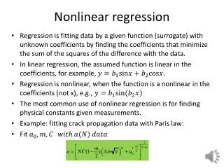
Exercise • The enzyme chymosin, which is found in the digestive tract of ruminants (Wiederkäuer) or produced recombinantly in E. Coli, is used in cheese production to destabilize the micelles in milk and make them aggregate. The following model is used to describe the kinetics of this process: Where y is the dimensionless concentration of stable micelles, z is the dimensionless concentration of destabilized micelles and A, B and C are parameters. The initial conditions (at t = 0 when the chymosin is added) are y = 1, z = 0. Daniel Baur / Numerical Methods for Chemical Engineers / Nonlinear Regression II
Assignment • Find online the data file milk.dat, which contains measurements of the change in the concentration of destabilized micelles over time, along with some code to import it into Matlab. • Plot the experimental data. • Write an ODE function that describes the system. Use a function of the form: • function dx = milkKinetics(t, x, A, B, C) • where x(1) will be the concentration of the stable micelles and x(2) will be the concentration of the destabilized micelles. Daniel Baur / Numerical Methods for Chemical Engineers / Nonlinear Regression II
Assignment (Continued) • Write a model function that returns the values predicted by the model for given parameters A, B and C and a time vector. Use a function of the form: • function yfit = milkModel(beta, time) • where A = beta(1), B = beta(2) and C = beta(3) • Inside this function, call an ode solver that solves the milkKinetics function, using as initial conditions x0 = [1; 0] and as time span the vectortime: • [time, y] = ode45(@(t,x)milkKinetics...); • yfit = y(:,2); • Test various values of A, B and C by solving the ODE system. How do the individual parameters influence the solution? • Hint: A is between 0.1 and 1, B is around 0.2 and C is between 5 and 50. Daniel Baur / Numerical Methods for Chemical Engineers / Nonlinear Regression II
Assignment (Continued) • Use either nlinfitor NonLinearModelto find a set parameters A, B, C that gives the best fit to the data in a least squares sense. Plot the resulting curves along with the data. Also determine the confidence intervals for the parameters and comment on the results.. • The modelfunction will simply read @milkModel. • The fitting process can take a few minutes, depending on the initial values. If the algorithm does not converge, call it again using the results of the non-converging run as initial guess. Daniel Baur / Numerical Methods for Chemical Engineers / Nonlinear Regression II