Download

1 / 69
700 likes | 849 Vues
This paper explores advanced motion planning strategies for autonomous mobile robots tasked with visual data collection in complex environments. Key applications include efficient map construction, target finding, and tracking, while considering both collision and visibility constraints. Utilizing a Randomized Next-Best-View motion planning algorithm, it addresses how robots should navigate to optimize sensing operations and dynamic target engagement. The paper highlights techniques for constructing 2D layouts, acquiring point data, and managing safe spaces, with applications in areas such as surveillance and architectural modeling.

E N D
Motion Planning with Visibility Constraints Jean-Claude Latombe Computer Science Department Stanford University
Main Collaborators • Hector Gonzalez • Steve LaValle • David Lin • Eric Mao • T.M. Murali • Leo Guibas • Cheng-Yu Lee • Rafael Murrieta
Autonomous Observer Mobile robot that performs visual data-collection tasks autonomously in complex environments, e.g.: • Construct a map/model of an environment • Find and track a moving target among obstacles
Map Building • A robot or a team of robots is introduced in an unknown environment • Where should the robot(s) successively go in order to build a map/model of the environment as efficiently as possible?
Target Finding • An evasive target hides in an environment with obstacles • A map of the environment is available • How should a robot or a team of robots move to sweep the building and eventually find the target?
Target Tracking • An evasive target is initially in the field of view of a robot, but may escape behind an obstacle. • A map of the environment is available. • How should the robot or the team of robots move to keep the target in the field of view of at least one robot at each time?
Core Problem Motion planning with both collision and visibility constraints
Some Applications • Intelligent camera • Telepresence, cooperation of geographically dispersed groups • 4D modeling of buildings • Automatic inspection of large structures • Architectural/archeological modeling • Surveillance and monitoring of plants • Military scouting
I. Map Building • Goal:Efficiently build a polygonal layout of an indoor environment • Question:Where should the robot go to perform the next sensing operation? • Approach:Randomized Next-Best View (NBV) motion planning algorithm
Why a Polygonal Layout? • Convenient to compute navigation paths and to extract topological information • Allows visibility computation • Compact model facilitating data exchanges, such as wireless communication among robots • Possibility of inserting uncertainty information
Robot Hardware • Nomadic Super-Scout wheeled platform • Sick laser range sensor mounted horizontally • 30 scans/s (180-dg scan, 360 pt/scan)
Construction of 2D Layouts • Go to successive sensing positions q1, q2, …, until the safe space F has no free edge • At each position qk, let M = (P,F) be the partial layout constructed so far. Do: • Acquire a list L of points • Transform L into a set p of polylines • Align P with p • Compute the safe space f corresponding to p • Compute the new safe space as the union of F and f
Construction of 2D Layouts • Go to successive sensing positions q1, q2, …, until the safe space F has no free edge • At each position qk, let M = (P,F) be the partial layout constructed so far. Do: • Acquire a list L of points • Transform L into a set p of polyline • Align P with p • Compute the safe space f corresponding to p • Compute the new safe space as the union of F and f
Construction of 2D Layouts • Go to successive sensing positions q1, q2, …, until the safe space F has no free edge • At each position qk, let M = (P,F) be the partial layout constructed so far. Do: • Acquire a list L of points • Transform L into a set p of polylines • Align P with p • Compute the safe space f corresponding to p • Compute the new safe space as the union of F and f
Construction of 2D Layouts • Go to successive sensing positions q1, q2, …, until the safe space F has no free edge • At each position qk, let M = (P,F) be the partial layout constructed so far. Do: • Acquire a list L of points • Transform L into a set p of polylines • Align P with p • Compute the safe space f corresponding to p • Compute the new safe space as the union of F and f
Alignment of Two Sets of Polylines • Pick two edges from smallest set at random • Match against two edges with same angle in other set • Evaluate quality of fit
Construction of 2D Layouts • Go to successive sensing positions q1, q2, …, until the safe space F has no free edge • At each position qk, let M = (P,F) be the partial layout constructed so far. Do: • Acquire a list L of points • Transform L into a set p of polylines • Align P with p • Compute the safe space f corresponding to p • Compute the new safe space as the union of F and f
Computed Safe Spaces normal exaggerated
Construction of 2D Layouts • Go to successive sensing positions q1, q2, …, until the safe space F has no free edge • At each position qk, let M = (P,F) be the partial layout constructed so far. Do: • Acquire a list L of points • Transform L into a set p of polylines • Compute the safe space f corresponding to p • Align P with p • Merge M and (p,f) by taking the union of F and f
Side-Effects of Merging Technique Detection, elimination, and separate recording of: • Transient objects • Small objects
Dealing with Small Objects • Detect spikes in the safe space f • Record the “apex” -- a small edge segment -- into a separate small-object map
Next-Best View Algorithm • Let M=(P,F) be the current partial layout. • Pick many points qi at random in F • Discard every qi if length of edges in P visible from qiis below a certain threshold (for reliable alignment) • Measure goodness of each qi as function of both amount of new space potentially visible from qi (through free edges) and length of shortest path (within F, avoiding small obstacles) from robot’s current position to qi • Select best qi as next sensing position
II. Target Finding • Goal:Find a target that is hiding in an environment cluttered with obstacles • Questions:How many robots are needed? How they should sweep the environment? • Approach:Cell decomposition of an information state
Assumptions • Target is unpredictable and can move arbitrarily fast • Environment is polygonal, with or without holes • Target and robots are modeled as point objects • A robot finds the target when the line segment connecting them does not intersect any obstacles
Related Work • Art-Gallery problems:O’Rourke, 1987; many others • Pursuit-evasion games:Isaacs, 1965; Hajek, 1975; Basar and Olsder, 1982; many others • Pursuit-evasion in a graph:Parsons, 1976; Megiddo et al., 1988; Lapaugh, 1993 • Pursuit-evasion in a simple polygon:Suzuki and Yamashita, 1992
Results • Lower bounds on the minimum number of robots N needed in environment with n edges and h holes • NP-hardness of computing N in given environment • Complete planner in environments searchable by one robot. Planner is rather fast in practice, but its worst-case running time is exponential in n • Greedy algorithm for environments requiring multiple robots. But no guarantee of optimality for number of robots • Extensions: cone of vision, aerial robot
Effect of Number n of Edges Minimal number of robotsN = O(log n)
Effect of Number n of Edges Minimal number of robotsN = Q(log n)
Effect of Number h of Holes N = Q(sqrt(h))
Two robots are needed Effect of Geometry on # of Robots
Conservative Cells In each conservative cell the set of visible edges remain constant
0 : the target does not hide beyond the edge 1 : the target may hide beyond the edge Information State Example of an information state = (1,1,0)
Search Graph • {Nodes} = {Conservative Cells} X {Information States} • Node (c,i) is connected to(c’,i’) iff: • Cells c and c’ share an edge (i.e., are adjacent) • Moving from c, with state i, into c’ yields state i’ • Initial node(c,i) is such that: • c is the cell where the robot is initially located • i = (1, 1, …, 1) • Goal node is any node where the information state is (0, 0, …, 0) Size is exponential in the number of edges in workspace
Visible Clear Contaminated Example of Target-Finding Strategy
Visible Clear Contaminated Example of Target-Finding Strategy