Download

1 / 84
840 likes | 997 Vues
This paper presents an innovative algorithm for solving the Single-Source Shortest Paths (SSSP) problem in graphs with positive integer weights in linear time. Traditional methods, such as Dijkstra’s algorithm, rely on sorting and have time complexities of O(n^2 + m). Our approach circumvents the sorting bottleneck by utilizing a hierarchical bucketing structure that enables efficient vertex visits in any order. This method improves computational efficiency and represents a significant advancement in algorithm design for graph theory.

E N D
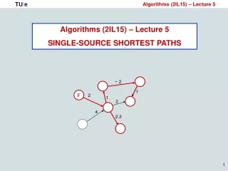
Undirected Single-Source Shortest Paths with Positive Integer Weights in Linear Time MIKKEL THORUP 1999 Journal of ACM
Presenters • 資工四 陳代樾 • 資工四 張愈敏 • 資工四 胡升鴻 • 資工四 呂哲安 • 資工四 陳縕儂 • 資工四 黃鈞愷
Outline • Introduction • Preliminary • Avoiding the Sorting Bottleneck • The Component Hierarchy • Visiting Minimal Vertices • Towards Linear Time • The Component Tree
Introduction(1) • MikkelThorup • http://www.diku.dk/~mthorup/
Introduction(2) Single SorceShortest Path Problem (SSSP) • Given a positively weighted graph G with a source vertex s, find the shortest path from s to all other vertices in the graph
Introduction(3) • Since 1959, all developments in SSSP have been based on Dijkstra’s algorithm O(n2 + m) • Our target is toward linear time and linear space algorithm. • The algorithm avoids the sorting bottleneck by building a hierarchical bucketing structure, identifying vertex pairs that may be visited in any order.
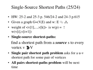
1 a b 4 4 c 2 1 7 e 4 d 1 1 f 3 g i h 1 4 Introduction(4) min 7 7 9 8 ∞ 8 min 11 9 9 ∞ min min Initial ∞ 8 8 8 ∞ 8 min 7 ∞ 7 min 0 4 4 5 5 ∞ min min Non-Decreasing Order
Introduction(5) • Notation: G = (V, E) | v | = n , | E | = m weighted function l : edge positive integer If (v, w) ∉ E , define l(v, w) = ∞ d(v) : distance from s to v D(v) : super distance D(v) ≧ d(v)
Introduction(6) • For each vertex we have We have a set such that and
Introduction(7) In fact, Dijkstra’s algorithm can be implemented in linear time linear time sorting Since we do not know how to sort in linear time, this implies that we are deviating from Dijkstra’s algorithm in that we do not visit the vertices in order of increasing distance from s • Our algorithm is based on a hierarchical bucketing structure. may visit the vertices in any order
Outline • Introduction • Preliminary • Avoiding the Sorting Bottleneck • The Component Hierarchy • Visiting Minimal Vertices • Towards Linear Time • The Component Tree
Preliminary(1) • Lemma 1. If v ∈ V\S minimize D(v) , D(v) = d(v) Proof: D(v) ≥ d(v) ≥ d(u) = D(u) ≥ D(v) • Lemma 2. • min D(V\S) = min d(V\S) is non-decreasing
Preliminary(2) • Notation: x >> i : x / 2i If x ≦ y => x >> i≦ y >> i If W ⊆ V , min D(W) >> i : (min{ D(w) | w ∈ W }) >> i
Preliminary(3) • Bucket • which elements can be inserted and deleted, and from which we can pick out an unspecified element. • each operation should be supported in O(1).
Outline • Introduction • Preliminary • Avoiding the Sorting Bottleneck • The Component Hierarchy • Visiting Minimal Vertices • Towards Linear Time • The Component Tree
Avoiding the Sorting Bottleneck(1) • Dijkstra’s algorithm • visit the vertices in order of increasingD(v) • Sorting bottleneck • New approach • visit the vertices where D(v) = d(v) , but possibly D(v) > min D(V\S) • Using bucket to maintain
Avoiding the Sorting Bottleneck(2) Lemma 3. Suppose the vertex set V divides into disjoint subsets V1, … , Vk and all edges between the subsets have length at least δ. Further suppose for some i, v ∈ Vi\S that D(v)=min D(Vi\S) ≦min D(V\S)+δ. Then d(v)=D(v).
0 1 4 ∞ ∞ 1 ∞ δ 7 ∞ ∞ 4 4 V2 V3 2 1 V1 7 4 1 1 3 1 4 Avoiding the Sorting Bottleneck(3) • For some i, v ∈ Vi\S,D(v) = min D(Vi\S)≦ min D(V\S) + δ i=3, δ =1 • Then, d(v) = D(v)
Avoiding the Sorting Bottleneck(4) • Criteria on D(v) = d(v): D(v) = min D(Vi\S) ≦ min D(V\S) + δ min D(Vi\S) ≦ min D(V\S) + 2α min D(Vi\S) >> α ≦ min D(V\S) >> α
Avoiding the Sorting Bottleneck(5) Bucket number: ∆+2 【Δ = Σe l(e) >> α】 bucket each i∈{1, . . . , k} according to min D(Vi\S) >>α. i belongs in bucket B(min D(Vi\S) >> α) Index: min D(Vi\S) >> α Content: i : 1,2,…,k Ix: smallest index of a nonempty bucket j i … content … ∞ 3 1 2 4 0 index ix Δ+ 2
j i … content … ∞ 3 1 2 4 0 index ix Δ+ 2 Avoiding the Sorting Bottleneck(6) • supposeixis maintained as the smallest index of a nonempty bucket • If i ∈ B(ix) and v ∈ Vi\S minimizes D(v), then D(v) = min D(Vi\S) ≦min D(V\S) +δ , so D(v) = d(v) by Lemma 3, and hence v can be visited
0 1 4 ∞ ∞ 1 ix ∞ δ 7 ∞ ∞ 4 4 5 V2 V3 2 1 V1 7 4 1 1 3 1 4 Avoiding the Sorting Bottleneck(7) δ = 20 , α = 0 B(min D(Vi\S) >> α) = i min D(V\S) = min d(V\S) is nondecreasing … … 3 2 3 1 … … ∞ 7 0 1 5 4 6 …
Outline • Introduction • Preliminary • Avoiding the Sorting Bottleneck • The Component Hierarchy • Visiting Minimal Vertices • Towards Linear Time • The Component Tree
Component Hierarchy(1) Introduction • Gi:the subgraph of G with l(e) < 2i • [v]i:the connected component on level i containing v • children of [v]i:[w]i-1, w ∈ [v]i 1 4 4 [v]1 2 1 7 4 v 1 1 w [w]1 3 [v]2 v 1 4 G0 G1 G3=G G2
Component Hierarchy(2) Introduction • [v]i is a min-child of [v]i+1if min D([v]i-) >> i = min D([v]i+1-) >> i • [v]iis minimal if [v]j is a min-child of [v]j+1 for j = i, …, b-1
Component Hierarchy(3) • Dijkstra’s algorithm visit v, if v ∈ V\S minimizes D(v) • For all i , min D([v]i-) >> i = min D([v]i+1-) >> i = D(v) >> i [v]0 minimal • min D(v) = d(v) [v]0 minimal • D(v) = d(v) [v]0 minimal
Component Hierarchy(4) • Lemma 5. If v ∉ S ,[v]iis minimal, and i ≤ j ≤ w, min D([v]i-) >> j-1 = min D([v]j-) >> j-1 . if j = i trivial if j > i, min D([v]i-) >> j - 1 = min D([v]j-1-) >> j - 1 = min D([v]j-) >> j - 1 .
Component Hierarchy(5) • Lemma 8. If v ∉ S and [v]iis minimal, min D([v]i-) = min d([v]i-). In particular, D(v) = d(v) if [v]0 = {v} is minimal. • Lemma 6. Suppose v ∉ S and there is a shortest path to v where the first vertex u outside S is in [v]i . Then d(v) ≥ min D([v]i-) . • Lemma 7. Suppose v ∉ S and [v]i+1 is minimal. If there is no shortest path to v where the first vertex outside S is in [v]i . Then d(v) >> i > min D([v]i+1-) >> i .
Component Hierarchy(6) • Lemma 6. Suppose v ∉ S and there is a shortest path to v where the first vertex u outside S is in [v]i . Then d(v) ≥ min D([v]i-) . u is th first vertex outside S D(u) ≤ d(v) u ∈ [v]i- d(v) ≥ D(u) ≥min D([v]i-)
Component Hierarchy(7) • Lemma 7. Suppose v ∉ S and [v]i+1 is minimal. If there is no shortest path to v where the first vertex outside S is in [v]i . Then d(v) >> i > min D([v]i+1-) >> i . If u ∉ [v]i+1, d(v) >> i + 1 > min D([v]i+2-) >> i + 1 = min D([v]i+1-) >> i+1 (induction) d(v) >> i> min D([v]i+1-) >> i If u ∈ [v]i+1, D(u) >> i≥ min D([v]i+1-) >> i but u ∉ [v]i, dist(u , v) ≥ 2i. d(v) >> i= (D(u)+ dist(u , v)) >> i ≥ min D([v]i+1-) >> i + 1
Component Hierarchy(8) • Lemma 8. If v ∉ S and [v]iis minimal, min D([v]i-) = min d([v]i-). In particular, D(v) = d(v) if [v]0 = {v} is minimal. D(w) ≥d(w) for all w min D([v]i-) ≥min d([v]i-) v is an arbitrary vertex in [v]i, show that d(v)≥ min D([v]i-) If u ∈ [v]i Lemma 6 If u ∉ [v]i Lemma 7 d(v) ≫ i> min D([v]i+1-) ≫ i . = min D([v]i-) ≫ i
Outline • Introduction • Preliminary • Avoiding the Sorting Bottleneck • The Component Hierarchy • Visiting Minimal Vertices • Towards Linear Time • The Component Tree
Visiting Minimal Vertices (1) • Definition • visiting a vertex requires that [v]0 = {v} is minimal • when v is visited, v is moved to S and relax • Lemma 10. For all [v]i, max d([v]i\[v]i-) >> i-1 ≦ min d([v]i-) >> i-1 • By lemma 5 D(w) >> i – 1 = min D([w]0-) >> i – 1 = min D([w]i-) >> i – 1 • By lemma 8 D(w) = d(w) and min D([w]i-) = min d([w]i-) d(w) >> i – 1 = min d([v]i-) >> i – 1
Visiting Minimal Vertices (2) • Lemma 11. min D([v]i-) >> i = min d([v]i-) >> i, visiting w ∈ V\S changes min D([v]i-) >> i w ∈ [v]i- , and the change in min D([v]i-) >> i is increased by one min D([v]i-) = min d([v]i-) is nondecreasing
Visiting Minimal Vertices (3) • Lemma 12. • If [v]i is minimal, it remains minimal until min D([v]i-) >> i is increased. (min d([v]i-) >> i is increased) • min D([v]i-) >> i = min D([v]i+1-) >> i • j is the smallest number such that [v]j+1 is minimal (j ≥ i) 〈e〉b and 〈e〉a denote the expression e should be evaluated before or after the event of visiting some vertex 〈min d([v]i-) >> j〉a ≥〈min d([v]j-) >> j〉a(j ≥ i) >〈min D([v]j+1-) >> j〉a(Lemma 9) ≥〈min D([v]j+1-) >> j〉b(nondecreasing) =〈min D([v]i-) >> j〉b([v]iis minimal) =〈min d([v]i-) >> j〉b([v]iis minimal)
Visiting Minimal Vertices (4) • Lemma 13. • If [v]i has once been minimal, in all future, min D([v]i-) >> i = min d([v]i-) >> i. • First time [v]i turns minimal (by lemma 8) • Visiting some vertex w • [v]i is minimal (by lemma 8) • [v]i is nonminimal (lemma 11, 12, D(v) ≥ d(v)) • [v]i- is emptied (both D and d -> ∞)
Visiting Minimal Vertices (5) A recursive call for Visit([v]i) where [v]i is minimal
a Visiting Minimal Vertices (6) • Visit([g]3) • min D([h]2-) >> 2 = min D([g]3-) >> 2 • Visit([h]2) • min D([h]1-) >> 1 = min D([h]2-) >> 1 • Visit([h]1) • min D([h]0-) >> 0 = min D([h]1-) >> 0 • Visit([h]0) 7 ∞ 1 b ∞ 4 4 c 2 1 ∞ ∞ 7 e 4 d ∞ 1 1 f 2 0 g i h 1 4 s 4 ∞
Outline • Introduction • Preliminary • Avoiding the Sorting Bottleneck • The Component Hierarchy • Visiting Minimal Vertices • Towards Linear Time • The Component Tree
1 a b 4 4 c 2 1 7 e 4 d 1 1 f 2 g i h 1 4 g e a c h i b d f Towards Linear Time (1) • Component Tree Number of nodes ≤ 2n-1 l(e) < 23 l(e) < 22 l(e) < 21
Towards Linear Time (2) • Linear-Sized Bucket Structure for all children [w]h of [v]i, bucket [w]h in B([v]i, min D([w]h-) >> i - 1) • ix0([v]i) = min D([v]i) >> i – 1 = min d([v]i) >> i – 1 ix∞([v]i) = ix0([v]i) + ∆([v]i) ≥ max d([v]i) >> i – 1 [v]i ix([v]i) =min D([v]i) >> i -1 ∑ l(e)/ 2i-1 content index
Towards Linear Time (3) • Lemma 18. The total number of relevant bucket is < 4m + 4n
Towards Linear Time (4) Visit([v]i, j)
Towards Linear Time (4) Visit([v]i, j) Visit(v)
Towards Linear Time (4) Visit([v]i, j)
Towards Linear Time (4) Expand([v]i) [v]i Min D([v]i) >> i - 1 ix0([v]i) + ∆([v]i)
Towards Linear Time (4) Visit([v]i, j)
1 a b 4 4 c 2 1 7 e 4 d 1 1 f 3 g i h 1 4 g e a c h i b d f Towards Linear Time (4) • ∞ 7 • Source: g • S ← {g} • Visit([g]3) • ∞ • ∞ • ∞ • ∞ • ∞ 0 4 [g]3 ∆([g]3) = 33 >> 2 = 8
1 a b 4 4 c 2 1 7 e 4 d 1 1 f 3 g i h 1 4 g e a c h i b d f Towards Linear Time (4) • ∞ 7 • Source: g • S ← {g} • Visit([g]3) • ∞ • ∞ • ∞ • ∞ • ∞ 0 4 [g]3 ∆([g]3) = 33 >> 2 = 8