Synchronous Computations
Synchronous Computations. In a (fully) synchronous computation, all the processes synchronized at regular points, usually to exchange data before proceeding. 6. 1. ITCS 4/5145 Parallel computing, UNC-Charlotte, B. Wilkinson Jan 23, 2013. Barrier.

Synchronous Computations
E N D
Presentation Transcript
Synchronous Computations In a (fully) synchronous computation, all the processes synchronized at regular points, usually to exchange data before proceeding. 6.1 ITCS 4/5145 Parallel computing, UNC-Charlotte, B. Wilkinson Jan 23, 2013
Barrier A basic mechanism for synchronizing processes - inserted at the point in each process where it must wait. All processes can continue from this point when all the processes have reached it (or, in some implementations, when a stated number of processes have reached this point). 6.2
In message-passing systems, barriers provided with library routines: 6.3
MPI MPI_Barrier() Barrier with a named communicator being the only parameter. Called by each process in the group, blocking until all members of the group have reached the barrier call and only returning then. 6.4
Internal Implementation of a Barrier routine Centralized counter implementation (a linear barrier): 6.5
Reentrant code Good barrier implementations must take into account that a barrier might be used more than once in a process. Might be possible for a process to enter the barrier for a second time before previous processes have left the barrier for the first time. Counter-based barriers often have two phases: • A process enters arrival phase and does not leave this phase until all processes have arrived in this phase. • Then processes move to departure phase and are released. Two-phase handles the reentrant scenario. 6.6
Barrier implementation in a message-passing system 6.7
Tree Implementation More efficient. O(log p) steps Suppose 8 processes, P0, P1, P2, P3, P4, P5, P6, P7: 1st stage: P1 sends message to P0; (when P1 reaches its barrier) P3 sends message to P2; (when P3 reaches its barrier) P5 sends message to P4; (when P5 reaches its barrier) P7 sends message to P6; (when P7 reaches its barrier) 2nd stage: P2 sends message to P0; (P2 & P3 reached their barrier) P6 sends message to P4; (P6 & P7 reached their barrier) 3rd stage: P4 sends message to P0; (P4, P5, P6, & P7 reached barrier) P0 terminates arrival phase; (when P0 reaches barrier & received message from P4) Release with a reverse tree construction. 6.8
Tree barrier 6.9
Butterfly Barrier 6.10
Local Synchronization and Data Transfer Suppose a process Pi needs be synchronized and exchange data with process Pi-1. Could consider: Need synchronous send()’s if synchronization as well as data transfer. Not a perfect three-process barrier because process Pi-1 will only synchronize with Pi and continue as soon as Pi allows. Similarly, process Pi+1 only synchronizes with Pi. 6.11
Safety and Deadlock When all processes send their messages first and then receive all of their messages is “unsafe” because it relies upon buffering in the send()s. The amount of buffering is not specified in MPI. If insufficient storage available, send routine may be delayed from returning until storage becomes available or until the message can be sent without buffering. Then, a locally blockingsend() could behave as a synchronous send(), only returning when the matching recv() is executed. Since a matching recv() would never be executed if all the send()s are synchronous, deadlock would occur. 6.12
Making the code safe Alternate the order of the send()s and recv()s in adjacent processes so that only one process performs the send()s first. Then even synchronous send()s would not cause deadlock. Example Linear pipeline, deadlock can be avoided by arranging so the even-numbered processes perform their sends first and the odd-numbered processes perform their receives first. Good way you can test for safety is to replace message-passing routines in a program with synchronous versions. 6.13
MPI Safe Message Passing Routines MPI offers several methods for safe communication: 6.14
Combined deadlock-free blocking sendrecv() routines MPI provides MPI_Sendrecv()and MPI_Sendrecv_replace(). (with12 parameters!) 6.15
MPI_Sendrecv() Combines blocking send with blocking receive operation without deadlock Source and destination can be the same or different. int MPI_Sendrecv( void *sendbuf, int sendcount, MPI_Datatype sendtype, int dest, int sendtag, void *recvbuf, int recvcount, MPI_Datatype recvtype, int source, int recvtag, MPI_Comm comm, MPI_Status *status) } Parameters for send Parameters for receive Same communicator 6.16
Synchronized Computations Can be classififed as: • Fully synchronous or • Locally synchronous In fully synchronous, all processes involved in the computation must be synchronized. In locally synchronous, processes only need to synchronize with a set of logically nearby processes, not all processes involved in the computation 6.17
Fully Synchronized Computation Examples Data Parallel Computations Same operation performed on different data elements simultaneously; i.e., in parallel. Particularly convenient because: • Ease of programming (essentially only one program). • Can scale easily to larger problem sizes. • Many numeric and some non-numeric problems can be cast in a data parallel form. Used in GPU’s see later in course. 6.18
Example To add the same constant to each element of an array: for (i = 0; i < n; i++) a[i] = a[i] + k; The statement a[i] = a[i] + k; could be executed simultaneously by multiple processors, each using a different index i (0<i<=n). 6.19
forall construct Special “parallel” construct to specify data parallel operations Example forall (i = 0; i < n; i++) { body } states that n instances of the statements of the body can be executed simultaneously. One value of the loop variable i is valid in each instance of the body, the first instance has i = 0, the next i = 1, and so on. To add kto each element of an array, a, we can write forall (i = 0; i < n; i++) a[i] = a[i] + k; 6.20
Data Parallel Example Prefix Sum Problem Given a list of numbers, x0, …, xn-1, compute all the partial summations, i.e.: x0+ x1; x0 + x1 + x2; x0 + x1 + x2 + x3; x0 + x1 + x2 + x3 + x4; … Can also be defined with associative operations other than addition. Widely studied. Practical applications in areas such as processor allocation, data compaction, sorting, and polynomial evaluation. 6.21
Sequential code for (j = 0, j < log(n); j++) /* at each step /* for (i = 2j; i < n; i++) /* accumulate sum */ x[i] = x[i] + x[i + 2j]; Parallel code using forall notation for (j=0, j< log(n); j++) /* at each step */ forall (i = 0; i < n; i++) /* accumulate sum */ if (i >= 2j) x[i] = x[i] + x[i + 2j]; 6.23
Synchronous Iteration (Synchronous Parallelism) Each iteration composed of several processes that start together at beginning of iteration. Next iteration cannot begin until all processes have finished previous iteration. Using forallconstruct: for (j = 0; j < n; j++) /*for each synch. iteration */ forall (i = 0; i < N; i++) { /*N procs each using*/ body(i); /* specific value of i */ } 6.24
Using message passing barrier: for (j = 0; j < n; j++) { /*for each synchr.iteration */ i = myrank; /*find value of i to be used */ body(i); barrier(mygroup); } 6.25
Another fully synchronous computation example Solving a General System of Linear Equations by Iteration Suppose the equations are of a general form with n equations and n unknowns where the unknowns are x0, x1, x2, … xn-1 (0 <= i < n). 6.26
By rearranging the ith equation: This equation gives xiin terms of the other unknowns. Can be be used as an iteration formula for each of the unknowns to obtain better approximations. 6.27
Jacobi Iteration All values of x are updated together. Can be proven that Jacobi method will converge if diagonal values of a have an absolute value greater than sum of the absolute values of the other a’s on the row (the array of a’s is diagonally dominant) i.e. if This condition is a sufficient but not a necessary condition. 6.28
Termination A simple, common approach. Compare values computed in one iteration to values obtained from the previous iteration. Terminate computation when all values are within given tolerance; i.e., when However, this does not guarantee the solution to that accuracy. 6.29
Convergence Rate 6.30
Parallel Code Process Pi could be of the form x[i] = b[i]; /*initialize unknown*/ for (iteration = 0; iteration < limit; iteration++) { sum = -a[i][i] * x[i]; for (j = 0; j < n; j++) /* compute summation */ sum = sum + a[i][j] * x[j]; new_x[i] = (b[i] - sum) / a[i][i]; /* compute unknown */ allgather(&new_x[i]); /*bcast/rec values */ global_barrier(); /* wait for all procs */ } allgather()sends the newly computed value of x[i]from process i to every other process and collects data broadcast from the other processes. 6.31
Introduce a new message-passing operation - Allgather. Allgather Broadcast and gather values in one composite construction. 6.32
Partitioning Usually number of processors much fewer than number of data items to be processed. Partition the problem so that processors take on more than one data item. block allocation – allocate groups of consecutive unknowns to processors in increasing order. cyclic allocation – processors are allocated one unknown in order; i.e., processor P0 is allocated x0, xp, x2p, …, x((n/p)-1)p, processor P1 is allocated x1, xp+1, x2p+1, …, x((n/p)-1)p+1, and so on. Cyclic allocation no particular advantage here (Indeed, may be disadvantageous because indices have to be computed in a more complex way and block data contiguous transfers are more efficient). 6.33
Locally Synchronous Computation Heat Distribution Problem An area has known temperatures along each of its edges. Find the temperature distribution within. 6.34
Divide area into fine mesh of points, hi,j. Temperature at an inside point taken to be average of temperatures of four neighboring points. Convenient to describe edges by points. Temperature of each point by iterating the equation: (0 < i < n, 0 < j < n) for a fixed number of iterations or until the difference between iterations less than some very small amount. 6.35
Heat Distribution Problem For convenience, edges also represented by points, but having fixed values, and used by computing internal values. 6.36
Number points from 1 for convenience and include those representing the edges. Each point will then use the equation Could be written as a linear equation containing the unknowns xi-m, xi-1, xi+1, and xi+m: Note: solving a (sparse) system Also solving Laplace’s equation, see later. 6.38
Sequential Code Using a fixed number of iterations for (iteration = 0; iteration < limit; iteration++) { for (i = 1; i < n; i++) for (j = 1; j < n; j++) g[i][j] = 0.25*(h[i-1][j]+h[i+1][j]+h[i][j-1]+h[i][j+1]); for (i = 1; i < n; i++) /* update points */ for (j = 1; j < n; j++) h[i][j] = g[i][j]; } using original numbering system (n x n array). 6.39
To stop at some precision: do { for (i = 1; i < n; i++) for (j = 1; j < n; j++) g[i][j] = 0.25*(h[i-1][j]+h[i+1][j]+h[i][j-1]+h[i][j+1]); for (i = 1; i < n; i++) /* update points */ for (j = 1; j < n; j++) h[i][j] = g[i][j]; continue = FALSE; /* indicates whether to continue */ for (i = 1; i < n; i++)/* check each pt for convergence */ for (j = 1; j < n; j++) if (!converged(i,j) { /* point found not converged */ continue = TRUE; break; } } while (continue == TRUE); 6.40
Parallel Code With fixed number of iterations, Pi,j (except for the boundary points): Important to use send()s that do not block while waiting for recv()s; otherwise processes would deadlock, each waiting for a recv() before moving on - recv()s must be synchronous and wait for send()s. 6.41
Version where processes stop when they reach their required precision: 6.42
Partitioning Normally allocate more than one point to each processor, because many more points than processors. Points could be partitioned into square blocks or strips: Communication on 4 edges Communication on 2 edges In general, strip partition best for large communication startup time, and block partition best for small startup time – see textbook for analysis 6.44
Ghost Points Additional row of points at each edge that hold values from adjacent edge. Each array of points increased to accommodate ghost rows. 6.45
Application Example A room has four walls and a fireplace. Temperature of wall is 20°C, and temperature of fireplace is 100°C. Write a parallel program using Jacobi iteration to compute the temperature inside the room and plot (preferably in color) temperature contours at 10°C intervals. 6.46
Other fully synchronous problems Cellular Automata The problem space is divided into cells. Each cell can be in one of a finite number of states. Cells affected by their neighbors according to certain rules, and all cells are affected simultaneously in a “generation.” Rules re-applied in subsequent generations so that cells evolve, or change state, from generation to generation. Most famous cellular automata is the “Game of Life” devised by John Horton Conway, a Cambridge mathematician. 6.48
The Game of Life Board game - theoretically infinite two-dimensional array of cells. Each cell can hold one “organism” and has eight neighboring cells, including those diagonally adjacent. Initially, some cells occupied. The following rules apply: 1. Every organism with two or three neighboring organisms survives for the next generation. 2. Every organism with four or more neighbors dies from overpopulation. 3. Every organism with one neighbor or none dies from isolation. 4. Each empty cell adjacent to exactly three occupied neighbors will give birth to an organism. These rules were derived by Conway “after a long period of experimentation.” 6.49
Simple Fun Examples of Cellular Automata “Sharks and Fishes” An ocean could be modeled as a three-dimensional array of cells. Each cell can hold one fish or one shark (but not both). Fish and sharks follow “rules.” 6.50