Test generation
Explore gate-level and high-level test generation techniques, including exhaustive, pseudo-exhaustive, and structural methods for verifying and testing digital circuits. Understand fault sensitization, path activation, and output function verification.

Test generation
E N D
Presentation Transcript
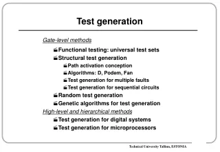
Test generation Gate-level methods • Functional testing: universal test sets • Structural test generation • Path activation conception • Algorithms: D, Podem, Fan • Test generation for multiple faults • Test generation for sequential circuits • Random test generation • Genetic algorithms for test generation High-level and hierarchical methods • Test generation for digital systems • Test generation for microprocessors
Test generation Universal test sets 1. Exhaustive test (trivial test) 2. Pseudo-exhaustive test Properties of exhaustive tests 1. Advantages (concerning the stuck at fault model): - test pattern generation is not needed - fault simulation is not needed - no need for a fault model - redundancy problem is eliminated - single and multiple stuck-at fault coverage is 100% - easily generated on-line by hardware 2. Shortcomings: - long test length (2n patterns are needed, n - is the number of inputs) - CMOS stuck-open fault problem
Test generation Output function verification Pseudo-exhaustive test sets: • Output function verification • maximal parallel testability • partial parallel testability • Segment function verification 4 4 4 Segment function verification 4 216 = 65536 >> 4x16 = 64 > 16 1111 0011 & F Pseudo- exhaustive sequential Pseudo- exhaustive parallel Exhaustive test 0101
Functional testing: universal test sets Output function verification (maximum parallelity) Exhaustive test generation for n-bit adder: Good news: Bit number n - arbitrary Test length - always 8 (!) Bad news: The method is correct only for ripple-carry adder 0-bit testing 1-bit testing 3-bit testing … etc 2-bit testing
Testing carry-lookahead adder General expressions: n-bit carry-lookahead adder:
Testing carry-lookahead adder R 1 1 0 0 1 1 0 0 1 1 0 0 1 1 0 0 1 1 0 0 1 1 0 0 1 1 1 1 1 0 0 1 1 1 1 1 1 0 0 1 1 0 1 1 1 1 1 0 1 1 0 1 1 0 1 1 1 0 1 1 1 0 0 1 1 1 1 0 1 1 1 1 0 1 1 0 1 0 1 1 1 1 1 0 0 1 1 0 1 1 1 1 1 1 0 0 Testing 0 Testing 1 For 3-bit carry lookahead adder for testing only this part of the circuit at least 9 test patterns are needed (i.e. pseudoexhaustive testing will not work) Increase in the speed implies worse testability
Test generation Output function verification (partial parallelity) F1 0011- - x1 F1(x1, x2) 0011- 0 F2(x1, x3) x2 010101 F3(x2, x3) F3 F4(x2, x4) x3 F2 010110 F5(x1, x4) F4 x4 00-11- F6(x3, x4) F5 000111 Exhaustive testing - 16 Pseudo-exhaustive, full parallel - 4 Pseudo-exhaustive, partially parallel - 6
Structural Test Generation Structural gate-level testing: fault sensitization: • A fault a/0 is sensitisized by the value 1 on a line a • A test t = 1101 is simulated, both without and with the fault a/0 • The fault is detected since the output values in the two cases are different • A path from the faulty line a is sensitized (bold lines) to the primary output
& & & Structural Test Generation • Fault sensitisation: • x7,1= D • Fault propagation: • x2=1, x1=1, b =1, c =1 • Line justification: • x7= D = 0: x3= 1, x4= 1 • b = 1: (already justified) • c = 1: (already justified) Structural gate-level testing: Path activation 1 1 Macro 1 d 1 1 a & 2 & 71 D D D 1 & e 3 7 72 b 1 1 4 y D D & 5 73 c 1 6 Test pattern Symbolic fault modeling: D = 0 - if fault is missing D = 1 - if fault is present
& & & Test generation Component F(x1,x2,…,xn) y Activate a path Test generation for a bridging fault: Bridge between leads 73 and 6 Wd Defect Macro 1 1 d 1 & 2 a & 71 D D • Fault manifestation: • Wd= x6x7= 1: x6= 0, x7= 1, • x7,1= D • Fault propagation: • x2= 1, x1= 1, b = 1, c = 1 • Line justification: • b = 1: x5= 0 D & e 3 72 7 b 1 4 y D D & 5 73 c 1 6 Wd
1 1 1 1 1 1 1 1 1 1 Test generation Multiple path fault propagation: 0 0 D D 0 0 x1 x1 D D 1 1 D x2 y x2 y D D 1 1 D D x3 x3 x4 x4 D 0 1 1 1 0 Three paths simultaneously activated Single path activation is not possible
Test generation D - algorithm (Roth, 1966): • Select a fault site, assign D • Propagate D along all available paths using D-cubes of gates • Backtracking, to find the inputs needed Example: Fault site D 1 D 1 & 2 4 1 Propagation D-cubes for AND-gate 3 1 1 D D & 4 2 1 3
Test generation D - algorithm: Propagation of D-cubes in the circuit: Primitive D-cubes for NAND and c 0: a b c 0 xD x 0 D Singular cover for C = NAND (A,B): a b c 1 1 0 x 0 1 0 x 1 4 1 & & 2 6 5 & • Intersection of cubes: • Let have 2 D-cubes • A = (a1, a2,... an) • B = (b1, b2,... bn) • where ai, bj 0,1,x,D,D) • 1) x ai = ai • 2) If ai x and bi x then • ai bi = ai if bi = ai or • ai bi = otherwise • 3) A B = if for any i: • ai bi = 3 1 2 3 4 5 6 D-drive: Primitive cube for x2 1 D Propagate D through G4 1 D D Propagate D through G6 1 D D 1 D Consistency operation: Intersect with G5 1 D 0 D 1 D Propagation D-cubes for C = NAND (A,B): a b c 1 DD D 1 D DDD
1 1 1 1 1 Test generation Multiple path fault propagation by DDs: Structural DD x41 x3 y x21 x12 x23 x33 x24 x42 x11 x31 x22 x32 0 Functional DD D 0 x1 D 1 x3 x1 x4 y x2 D x2 y 1 D x3 x3 x1 x4 x4 D 0 1 1 0
Test generation PODEM - algorithm (Goel, 1981): 1. Controllability measures are used during backtracking Decision gate: The “easiest” input will be chosen at first Imply gate: The “most difficult” input will be chosen at first 2. Backtracking ends always only at inputs 3. D-propagation on the basis of observability measures 0 0 & 1 & 1
Test generation FAN - algorithm (Fujiwara, 1983): 1. Special handling of fan-outs (by using counters) PODEM: backtracking continues over fan-outs up to inputs FAN: backtracking breaks off, the value is chosen on the basis of values in counters 2. Heuristics is introduced into D-propagation PODEM: moves step by step (without predicting problems) FAN: finds bottlenecks and makes appropriate decisions at the beginning, before starting D-propagation 1 (C = 6) Chosen value: 1 0 (C = 3) 0 (C = 2)
Example: Test Generation with SSBDDs Testing Stuck-at-0 faults on paths: x11 x21 1 y x11 x1 x21 & x2 x12 x31 x4 x12 x31 x3 y & 1 x4 Test pattern: x22 x32 x13 & x13 x1 x2 x3 x4 y 1 10- 1 & x22 x32 0 Tested faults: x120, x210
Example: Test Generation with SSBDDs Testing Stuck-at-0 faults on paths: x21 y x11 x1 & x2 x31 x4 x12 1 x3 y & 1 x4 x22 x32 x13 & & Test pattern: 0 x1 x2 x3 x4 y 1 0 1 1 1 Tested faults: x120, x310, x40
Example: Test Generation with SSBDDs Testing Stuck-at-0 faults on paths: x21 y x11 x1 & x2 x31 x4 x12 x3 y & 1 x4 x22 x32 x13 1 & & Test pattern: x1 x2 x3 x4 y 0 110 1 0 Tested faults: x220, x320 Not tested: x131
Example: Test Generation with SSBDDs Testing Stuck-at-1 faults on paths: y x21 x11 1 x11 x1 x21 & x2 x31 x4 x12 x12 1 x31 x3 y & 1 x4 x22 x32 x13 1 Test pattern: & x13 x1 x2 x3 x4 y 00110 & x22 0 x32 Tested faults: x121, x221 Not tested: x111
Example: Test Generation with SSBDDs Testing Stuck-at-1 faults on paths: y x21 x11 1 x11 x1 x21 & x2 x31 x4 x12 x12 1 x31 x3 y & 1 x4 x22 x32 x13 1 Test pattern: & x13 x1 x2 x3 x4 y 10010 & x22 0 x32 Tested faults: x211, x311, x130
Example: Test Generation with SSBDDs Testing Stuck-at-1 faults on paths: y x21 x11 1 x11 x1 x21 & x2 x31 x4 x12 x12 1 x31 x3 y & 1 x4 x22 x32 x13 1 Test pattern: & x13 x1 x2 x3 x4 y 10100 & x22 0 x32 Not yet tested fault: x321 Tested fault: x41
Transformation of BDDs y y y x2 x21 x2 x1 x11 x1 SSBDD: x3 x4 x31 x4 x31 x4 x12 x12 x12 x22 x32 x22 x32 x22 x32 x13 x13 x13 y x2 y x2 x1 x1 Optimized BDD: x4 x3 x4 x3 BDD: x2 x3 x2
Example: Test Generation with BDDs Testing Stuck-at faults on inputs: y x21 x11 x11 x1 x21 SSBDD: & x2 x31 x4 x12 x12 x31 x3 y & 1 x22 x32 x4 x13 & x13 y x2 x1 1 & x22 BDD: x32 x1 x2 x3 x4 y D10-D x4 x3 Test pair D=0,1: x2 0 Tested faults: x10, x11
Test generation Test generation by using disjunctive normal forms
Multiple Fault Testing Multiple faults fenomena: • Multiple stuck-fault (MSF) model is a straightforward extension of the single stuck-fault (SSF) model where several lines can be simultaneously stuck • If n - is the number of possible SSF sites, there are 2n possible SSFs, but there are 3n -1 possible MSFs • If we assume that the multiplicity of faults is no greater than k , then the number of possible MSFs is ki=1 {Cni}2i • The number of multiple faults is very big. However, their consideration is needed because of possible fault masking
Multiple Fault Testing Fault masking • Let Tg be a test that detects a fault g • A fault ffunctionally masks the fault g iff the multiple fault { f, g } is not detected by any pattern in Tg The test 011 is the only test that detects the fault c 0 The same test does not detect the multiple fault { c 0, a 1} Thus a 1 masks c 0 • Let Tg’T be the set of all tests in T that detect a fault g • A fault fmasks the fault g under a test T iff the multiple fault { f , g} is not detected by any test in Tg’ Example: Fault a 1 Fault c 0
Multiple Fault Testing Multiple fault F may be not detected by a complete test T for single faults because of circular masking among the faults in F Circular fault masking Example: • The test T = {1111, 0111, 1110, 1001, 1010, 0101} detects every SSF • The only test in T that detects the single faults b 1 and c 1 is 1001 • However, the multiple fault {b1, c1} is not detected because under the test vector 1001,b 1masks c 1, and c 1 masks b 1 1 a 1/0 & 0/1 b 1 & 0/1 0 & 0/1 & 0/1 1 c & 1 d 1/0
Multiple Fault Testing Testing multiple faults by pairs of patterns To test a path under condition of multiple faults, two pattern test is needed As the result, either the faults on the path under test are detected or the masking fault is detected Example: The lower path from b to output is under test A pair of patterns is applied on b There is a masking fault c 1 1st pattern: fault on b is masked 2nd pattern: fault on c is detected 11 10 a & 01 b 11 & 1 faults 01 (00) & 01 & 00 (11) 10 (11) c & 11 d 11(00) • The possible results: • 01 - No faults detected • 00 - Either b 0or c 1detected • 11 - The fault b 1isdetected
Test generation Testing multiple faults by groups of patterns Multiple fault:x11, x20, x31 An example where the method of test pairs does not help Fault masking Fault detecting T1 T2 T3 x31 x11 x20
Test generation Method of pattern groups on DDs x1 x2 y x1 & x2 Test group for testing a part of circuit: x3 x3 x4 y x1 & 1 x4 & x2 x3 x1 x2 x3 x4 y 1 1 0 - 1 0 1 0 - 0 1 0 0 - 0 - x1 & Disjunctive normal forms are trending to explode DDs provide an alternative
Test generation Test generation for sequential circuits Fault sensitization: Test pattern consists of an input pattern and a state Fault propagation: To propagate a fault to the output, an input pattern and a state is needed Line justification: To reach the needed state, an input sequence is needed y x CC R Time frame model: y x y y x x CC CC CC R R R
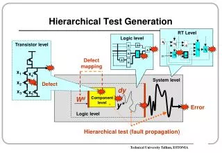
Hierarchical Test Generation • In high-level symbolic test generation the test properties of components are often described in form of fault-propagation modes • These modes will usually contain: • a list of controlsignals such that the data on input lines is reproduced without logic transformation at the output lines - I-path, or • a list of control signals that provide one-to-one mapping between data inputs and data outputs - F-path • The I-paths and F-paths constitute connections for propagating test vectors from input ports (or any controllable points) to the inputs of the Module Under Test (MUT) and to propagate the test response to an output port (or any observable points) • In the hierarchical approach, top-down and bottom-up strategies can be distinguished
Hierarchical Test Generation Approaches Bottom-up approach: Top-down approach: A A System System a a’ D D’ B B c’ C C c a’,c’,D’ fixed x - free a,c,D fixed x - free a a’x D d’x A = a’x D’ = d’x C = c’x A = ax D: B = bx C = cx c c’x Module Module
Hierarchical Test Generation Approaches A System Bottom-up approach: • Pre-calculated tests for components generated on low-level will be assembled at a higher level • It fits well to the uniform hierarchical approach to test, which covers both component testing and communication network testing • However, the bottom-up algorithms ignore the incompletenessproblem • The constraints imposed by other modules and/or the network structure may prevent the local test solutions from being assembled into a global test • The approach would work well only if the the corresponding testability demands were fulfilled a D B C c a,c,D fixed x - free a D A = ax D: B = bx C = cx c Module
Hierarchical Test Generation Approaches Top-down approach: A System • Top-down approach has been proposed to solve the test generation problem by deriving environmental constraints for low-level solutions. • This method is more flexible since it does not narrow the search for the global test solution to pregenerated patterns for the system modules • However the method is of little use when the system is still under development in a top-down fashion, or when “canned” local tests for modules or cores have to be applied a’ D’ B c’ C a’,c’,D’ fixed x - free a’x d’x A = a’x D’ = d’x C = c’x c’x Module
y y y y 1 2 3 4 a R · c 1 M + 1 e · M R 3 2 b · * M · 2 IN · d Test Generation High-level test generation with DDs: Conformity test Decision Diagram Multiple paths activation in a single DD Control function y3 is tested R 2 0 y # 0 4 Data path 1 R 2 0 0 2 y y R + R 3 1 1 2 1 IN + R 2 1 IN 2 R 1 3 0 y R * R 2 1 2 1 IN* R Control: For D = 0,1,2,3: y1 y2 y3 y4 = 00D2 Data: Solution of R1+ R1 IN R1 R1* R1 Test program: 2
y y y y 1 2 3 4 a R · c 1 M + 1 e · M R 3 2 b · * M · 2 IN · d Test Generation High-level test generation with DDs: Scanning test Decision Diagram Single path activation in a single DD Data function R1* R2is tested R 2 0 y # 0 4 Data path 1 R 2 0 0 2 y y R + R 3 1 1 2 1 IN + R 2 1 IN 2 R 1 3 0 y R * R 2 1 2 1 IN* R Control: y1 y2 y3 y4 = 0032 Data: For all specified pairs of (R1, R2) Test program: 2
Test Generation High-level path activation on DDs • Transparency functions • on Decision Diagrams: • Y = C y3 = 2, R2’ = 0 • C - to be tested • R1 = B y1 = 2, R3’ = 0 • R1 - to be justified
0 # 1001 q y1 y2 y3 q’ 1 1 #2120 R’ =0 2 0 # #3021 2 4200 # 3 4 # # 4211 0112 Test Generation DD synthesis for control path DD for the FSM: FSM state transitions and output functions
0 # 1001 q y1 y2 y3 q’ 1 1 #2120 R’ =0 2 0 # #3021 2 4200 # 3 4 # # 4211 0112 Test Generation High-level DDs Data path Control path
y # = 0 0 2 Test Generation for Digital Systems High-level test generation for data-path (example): t Time: t-1 t-2 t-3 q’=4 q’=2 q’=1 q’=0 y =2 3 y R’ = 0 = 0 2 2 R =D 3 # 0 R’ =0 2 q’=2 Fault propagation q’=1 y =2 • Test generation steps: • Fault manifestation • Fault-effect propagation • Constraints justification 1 y = 0 3 C =D R’ =0 A =D 3 1 # 0 * A R’ R’ =D B =D 1 1 2 2 Fault manifestation Constraints justification
y y 2 y 3 # A A R 2 s y 1 + R Y 3 B * F R C 1 = 0 0 # 4211 2 Test Generation for Digital Systems • Test generation step: • Fault-effect propagation t Time: t-1 t-2 t-3 q’=2 q’=1 q’=0 q’=4 0 y # y Y,R 0 =2 3 3 3 y R’ = 0 = 0 2 2 1 R =D R’ 3 3 2 # 0 q y1 y2 y3 0 R’ =0 C R’ 2 q’=2 0 2 # 1001 Fault propagation q’ q’=1 0 C R’ 1 1 y =2 2 #2120 R’ =0 1 2 y = 0 0 3 C =D R’ =0 # #3021 A =D 3 C+R’ 1 # 2 2 0 4200 # * A R’ R’ =D B =D 1 1 2 2 3 Fault manifestation 4 # 0112 Constraints justification
y # t Time: t-1 t-2 t-3 q’=4 q’=2 q’=1 q’=0 0 y # R 0 2 2 y =2 1 3 R’ y 2 R’ = 0 = 0 2 2 2 R =D A 3 # 0 3 2 = 0 R’ =0 2R’ 2 q’=2 2 Fault propagation q’=1 0 y =2 1 y 0 = 0 y # R 0 3 1 1 C =D R’ =0 A =D 3 1 1 # 0 R’ 1 2 * A R’ R’ =D B =D 0 1 1 2 2 B R’ 3 Fault manifestation F(B,R’ ) Constraints justification 3 # # 0112 4211 2 Test Generation for Digital Systems • Test generation step: • Line justification • Time: t-1 Path activation procedures on DDs: 0 0 # y Y,R 0 3 3 1 R’ 3 2 0 C R’ 2 0 C R’ 2 C+R’ 2 0 q y1 y2 y3 # 1001 q’ 1 1 #2120 R’ =0 2 0 # #3021 2 4200 # 3 4
y # = 0 0 2 Test Generation for Digital Systems High-level test generation example: t Time: t-1 t-2 t-3 Symbolic test sequence: q’=4 q’=2 q’=1 q’=0 y =2 3 y R’ = 0 = 0 2 2 R =D 3 # 0 R’ =0 2 q’=2 Fault propagation q’=1 y =2 1 y = 0 3 C =D R’ =0 A =D 3 1 # 0 * A R’ R’ =D B =D 1 1 2 2 Fault manifestation Constraints justification
I1: MVI A,D A IN I2: MOV R,A R A I3: MOV M,R OUT R I4: MOV M,A OUT IA I5: MOV R,M R IN I6: MOV A,M A IN I7: ADD R A A + R I8: ORA R A A R I9: ANA R A A R I10: CMA A,D A A Test Generation Test program generation for a microprocessor (example): DD-model of the microprocessor: Instruction set: 1,6 A I IN 3 2,3,4,5 I R OUT IN 4 7 A + R A 8 2 A R I A R 9 A R 5 IN 10 A 1,3,4,6-10 R
Test Generation Test program generation for a microprocessor (example): DD-model of the microprocessor: Scanning test for adder: Instruction sequence I5 I1 I7 I4 for all needed pairs of (A,R) 1,6 A I IN I4 3 OUT 2,3,4,5 I R OUT IN I7 A 4 7 A + R I1 A A 8 R IN(2) 2 A R I A R I5 R 9 A R 5 IN(1) IN Time: 10 t t - 1 t - 2 t - 3 A 1,3,4,6-10 Observation Test Load R
Test Generation Test program generation for a microprocessor (example): Conformity test for decoder: Instruction sequence I5 I1 DI4 for all DI1 -I10 at given A,R,IN DD-model of the microprocessor: 1,6 A I IN Data generation: 3 2,3,4,5 I R OUT IN 4 7 A + R A 8 2 A R I A R 9 A R 5 IN 10 A 1,3,4,6-10 Data IN,A,R are generated so that the values of all functions were different R
Test Generation Hierarchical approach with functional fault model: