CMB Polarization Results from the Cosmic Background Imager

2. CMB Polarization Results from the Cosmic Background Imager Steven T. Myers National Radio Astronomy Observatory Socorro, NM

3. The Cosmic Background Imager • A collaboration between • Caltech (A.C.S. Readhead PI, S. Padin PS.) • NRAO • CITA • Universidad de Chile • University of Chicago • With participants also from • U.C. Berkeley, U. Alberta, ESO, IAP-Paris, NASA-MSFC, Universidad de Concepción • Funded by • National Science Foundation, the California Institute of Technology, Maxine and Ronald Linde, Cecil and Sally Drinkward, Barbara and Stanley Rawn Jr., the Kavli Institute, and the Canadian Institute for Advanced Research

4. The CMB Landscape

5. Thermal History of the Universe Courtesy Wayne Hu – http://background.uchicago.edu

6. CMB Primary Anisotropies • Low l (<100) • primordial power spectrum (+ S-W, tensors, etc.) • Intermediate l (100-2000) • dominated by acoustic peak structure • position of peak related to sound crossing angular scale  angular diameter distance to last scattering • peak heights controlled by baryons & dark matter, etc. • damping tail roll-off with  • Large l (2000-5000+) • realm of the secondaries (e.g. SZE) Courtesy Wayne Hu – http://background.uchicago.edu

7. CMB Acoustic Peaks • Compression driven by gravity, resisted by radiation ≈ “j ladder” series of harmonics + projection corrections peaks: ~ plsj troughs: ~ pls (j±½)

8. Bond et al. 2002 • SPH (5123) [Wadsley et al. 2002] • MMH (5123) [Pen 1998] SZE Secondary 8=1.0, 0.9 CMB Secondary Anisotropies Courtesy Wayne Hu – http://background.uchicago.edu

9. CMB Polarization • Due to quadrupolar intensity field at scattering Courtesy Wayne Hu – http://background.uchicago.edu

10. CMB Polarization • E & B modes: translation invariance • E (gradient) from scalar density fluctuations predominant! • B (curl) from gravity wave tensor modes, or secondaries Courtesy Wayne Hu – http://background.uchicago.edu

11. Note: polarization peaks out of phase w.r.t. intensity peaks Polarization Power Spectrum Planck “error boxes” Hu & Dodelson ARAA 2002

12. The Gold Standard: WMAP + “ext” WMAP ACBAR

13. The Cosmic Background Imager

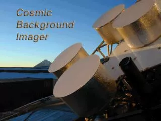
14. The Instrument • 13 90-cm Cassegrain antennas • 78 baselines • 6-meter platform • Baselines 1m – 5.51m • 10 1 GHz channels 26-36 GHz • HEMT amplifiers (NRAO) • Cryogenic 6K, Tsys 20 K • Single polarization (R or L) • Polarizers from U. Chicago • Analog correlators • 780 complex correlators • Field-of-view 44 arcmin • Image noise 4 mJy/bm 900s • Resolution 4.5 – 10 arcmin

15. Other CMB Interferometers: DASI, VSA • DASI @ South Pole • VSA @ Tenerife

16. CBI Site – Northern Chilean Andes • Elevation 16500 ft.!

17. The CBI Adventure… • Steve Padin wearing the cannular oxygen system • because you never know when you need to dig the truck out!

18. 3-Axis mount : rotatable platform

19. The CMB and Interferometry • The sky can be uniquely described by spherical harmonics • CMB power spectra are described by multipole l • For small (sub-radian) scales the spherical harmonics can be approximated by Fourier modes • The conjugate variables are (u,v) as in radio interferometry • The uv radius is given by |u| =l / 2p • An interferometer naturally measures the transform of the sky intensity in l space convolved with aperture

20. multipole: l = 2pB/λ = 2p|uij| shortest CBI baseline: central hole 10cm The uv plane • The projected baseline length gives the angular scale

21. primary beam transform: θpri= 45' Δl ≈ 4D/λ ≈ 360 mosaic beam transform: θmos= n×45' Δl ≈ 4D/nλ CBI Beam and uv coverage • Over-sampled uv-plane • excellent PSF • allows fast gridded method (Myers et al. 2000)

22. CBI 2000+2001, WMAP, ACBAR, BIMA • Readhead et al. ApJ, 609, 498 (2004) • astro-ph/0402359 SZE Secondary CMB Primary

23. CMB Interferometry

24. Rohlfs & Wilson Polarization of radiation • Electromagnetic Waves • Maxwell: 2 independent linearly polarized waves • 3 parameters (E1,E2,d)  polarization ellipse

25. The Poincare Sphere Rohlfs & Wilson Polarization of radiation • Electromagnetic Waves • Maxwell: 2 independent linearly polarized waves • 3 parameters (E1,E2,d)  polarization ellipse • Stokes parameters (Poincare Sphere): • intensity I (Poynting flux) I2= E12 + E22 • linear polarization Q,U (mI)2= Q2 + U2 • circular polarization V (vI)2= V2

26. Polarization of radiation • Electromagnetic Waves • Maxwell: 2 independent linearly polarized waves • 3 parameters (E1,E2,d)  polarization ellipse • Stokes parameters (Poincare Sphere): • intensity I (Poynting flux) I2= E12 + E22 • linear polarization Q,U (mI)2= Q2 + U2 • circular polarization V (vI)2= V2 • Coordinate system dependence: • I independent • V depends on choice of “handedness” • V > 0 for RCP • Q,U depend on choice of “North” (plus handedness) • Q “points” North, U 45 toward East • EVPA F = ½ tan-1 (U/Q) (North through East)

27. Polarization – Stokes parameters • CBI receivers can observe either RCP or LCP • cross-correlate RR, RL, LR, or LL from antenna pair • CMB intensity I plus linear polarization Q,U important • CMB not circularly polarized, ignore V (RR = LL = I) • parallel hands RR, LL measure intensity I • cross-hands RL, LR measure complex polarization P=Q+iU • R-L phase gives electric vector position angle F = ½ tan-1 (U/Q) • rotates with parallactic angle of detector y on sky

28. Polarization Interferometry • Parallel-hand & Cross-hand correlations • for antenna pair i, j and frequency channel n : • where kernel P is the aperture cross-correlation function • and y the baseline parallactic angle (w.r.t. deck angle 0°)

29. E and B modes • A useful decomposition of the polarization signal is into “gradient” and “curl modes” – E and B: E & B response smeared by phase variation over aperture A interferometer “directly” measures (Fourier transforms of) E & B!

30. Power Spectrum of CMB • Statistics of CMB field • Gaussian random field – Fourier modes independent • described by angular power spectrum • 4 non-zero polarization covariances: TT,EE,BB,TE (plus EB, TB)

31. fiducial power spectrum shape (e.g. 2p/l2) c=1 if l in band B; else c=0 projected noise fitted residual (statistical) foreground known foregrounds (e.g point sources) scan (ground) signal Power Spectrum and Likelihood • Break Cl into bandpowers qB: • Covariance matrix C sum of individual covariance terms: • maximize Likelihood for complex visibilities V:

32. CBI Polarization Data Processing • Massive data processing exercise • 4 mosaics, 300 nights observing • more than 106 visibilities total! • scan projection over 3.5° requires fine gridding • more than 104 gridded estimators • Method: Myers et al. (2003) • gridded estimators + max. likelihood • tested in CBI 2000, 2001-2002 papers • Parallel computing critical • both gridding and likelihood now parallelized using MPI • using 256 node/ 512 proc McKenzie cluster at CITA • 2.4 GHz Intel Xeons, gigabit ethernet, 1.2 Tflops! • currently 4-6 hours per full run (!) • current limitation 1 GB memory per node Matched filter gridding kernel mosaicing phase factor

33. w/o source projection (×½) Tests with mock data • The CBI pipeline has been extensively tested using mock data • Use real data files for template • Replace visibilties with simulated signal and noise • Run end-to-end through pipeline • Run many trials to build up statistics

34. Detail: leakage “true” signal • Leakage of R  L (d-terms): 2nd order: D•P into I 2nd order: D2•I into I 1st order: D•I into P 3rd order: D2•P* into P

35. CBI Polarization New Results! astro-ph/0409569 (24 Sep 2004) Brought to you by: A. Readhead, T. Pearson, C. Dickinson (Caltech) S. Myers, B. Mason (NRAO), J. Sievers, C. Contaldi, J.R. Bond (CITA) P. Altamirano, R. Bustos, C. Achermann (Chile) & the CBI team!

36. Carlstrom et al. 2003 astro-ph/0308478 2002 DASI & 2003 WMAP Polarization Courtesy Wayne Hu – http://background.uchicago.edu

37. New: DASI 3-year polarization results! • Leitch et al. 2004 (astro-ph/0409357) 16Sep04! • EE 6.3 σ • TE 2.9 σ • consistent w/ WMAP+ext model • BB consistent with zero • no foregrounds (yet)

38. New: DASI 3-year polarization results! • Leitch et al. 2004 (astro-ph/0409357) 16Sep04! • CMB thermal spectrum nbb=0 : found b=0.11±0.13 • vs. synchrotron b = -2.0 to -3.0 • no point sources seen in images (>15 mJy) • test against synchrotron (diffuse and point) foregrounds • relative to 8.5 mK2 at l = 300 • NO POLARIZED FOREGROUNDS DETECTED !

39. CBI Current Polarization Data • Observing since Sep 2002 (processed to May 2004) • compact configuration, maximum sensitivity

40. CBI Polarization Mosaics • Four mosaics a = 02h, 08h, 14h, 20h at d = 0° • 02h, 08h, 14h 6 x 6 fields, 20h deep strip 6 fields [45’ centers]

41. Before ground subtraction: • I, Q, U dirty mosaic images:

42. After ground subtraction: • I, Q, U dirty mosaic images (9m differences):

43. CBI Calibration & Foregrounds • Calibration on TauA (Crab) & Jupiter • use TauA to calibrate R-L phase (26 Jy of polarized flux!) • secondary calibrators also (3C274, Mars, Saturn, …) • Scan subtraction/projection • observe scan of 6 fields, 3m apart = 45’ • lose only 1/6 data to differencing (cf. ½ previously) • Point source projection • list of NVSS sources (extrapolation to 30 GHz unknown) • 3727 total for TT  many modes lost, sensitivity reduced • use 557 for polarization (bright OVRO + NVSS 3s pol) • need 30 GHz GBT measurements to know brightest

44. CBI Diffuse Foregrounds • Mid-High galactic latitudes (25°– 50° vs. 60° DASI) • Galactic cosmic rays (synchrotron emission) • from WMAP template (Bennett et al. 2003) • mean, rms, max not significantly worse than in DASI fields • except 14h field (in North Polar Spur) 50% worse • Rely on CBI frequency leverage (26-36 GHz) • synchrotron spectrum n-2.7 vs. thermal • also l2 vs. CMB in power spectrum

45. CBI & DASI Fields galactic projection – image WMAP “synchrotron” (Bennett et al. 2003)

46. New: CBI Polarization Power Spectra • 7-band fits (Dl = 150 for 600<l<1200) • bin positions well-matched to peaks & valleys • offset bins run also • narrower bins (Dl = 75) – scatter from F-1 • bin resolution limited by signal-to-noise

47. Data Tests • Test robustness to systematic effects, such as: • instrumental effects (amplitude, polarization) • foregrounds (synchrotron, free-free, dust) • Numerous c2 and noise tests • few discrepant days found  no difference to results • Conduct series of splits and “jack-knife” tests, e.g.: • primary vs. secondary calibrators (calibration consistency) • first half vs. second half of data (time-variable instrument) • “jack-knife” on antennas (bad single antenna) • “jack-knife” on fields (bad single field) • high vs. low frequency channels (e.g. foregrounds) NO SIGNIFICANT DEVIATIONS FOUND!

48. Shaped Cl fits • Use WMAP’03 best-fit Cl in signal covariance matrix • bandpower is then relative to fiducial power spectrum • compute for single band encompassing all ls • Results for CBI data (sources projected from TT only) • qB = 1.22 ± 0.21 (68%) • EE likelihood vs. zero : equivalent significance 8.9 σ • Conservative - project subset out in polarization also • qB = 1.18 ± 0.24 (68%) • significance 7.0 σ

49. New: CBI Polarization Parameters • use fine bins (Dl = 75) + window functions (Dl = 25) • cosmological models vs. data using MCMC • modified COSMOMC (Lewis & Bridle 2002) • Include: • WMAP TT & TE • WMAP + CBI’04 TT & EE (Readhead et al. 2004b = new!) • WMAP + CBI’04 TT & EE l <1000 + CBI’02 TT l >1000 (Readhead et al. 2004a) [overlaps ‘04]

50. New: CBI Polarization Parameters • use fine bins (Dl = 75) + window functions (Dl = 25) • Include: • WMAP TT & TE • CBI 2004 Pol TT, EE (Readhead et al. 2004b = new) • CBI 2001-2002 TT (Readhead et al. 2004a) • NOTE: parameter constraints dominated by higher precision TT from CBI 2001-2002 data!