Hidden Markov Models (1)
400 likes | 724 Vues
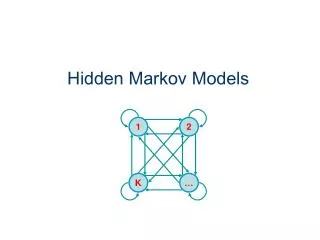
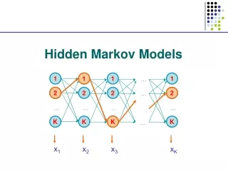
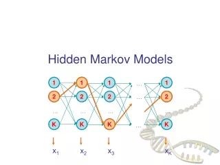
Basic Local Alignment Search Tool (BLAST). The strategy Important parameters Example Variations. Hidden Markov Models (1). Brief review of discrete time finite Markov Chain Hidden Markov Model Examples of HMM in Bioinformatics Estimations. BLAST.

Hidden Markov Models (1)
E N D
Presentation Transcript
Basic Local Alignment Search Tool (BLAST) • The strategy • Important parameters • Example • Variations Hidden Markov Models (1) • Brief review of discrete time finite Markov Chain • Hidden Markov Model • Examples of HMM in Bioinformatics • Estimations
BLAST “Basic Local Alignment Search Tool” Given a sequence, how to find its ‘relatives’ in a database of millions of sequences? An exhaustive search using pairwise alignment is impossible. BLAST is a heuristic method that finds good, but not necessarily optimal, matches. It is fast. Basis: good alignments should contain “words” that match each other very well (identical or with very high alignment score).
BLAST Pandit et al. In Silico Biology 4, 0047
BLAST • The scoring matrix: example:BLOSUM62 The expected score of two random sequences aligned to each other is negative. High scores of alignments between two random sequences follow the Extreme Value Distribution.
BLAST The general idea of the original BLAST: Find a match of words in a database. This is done efficiently using pre-processed database and hashing technique. Extend the match to find longer local alignments. Report results exceeding a predefined threshold.
BLAST Two key parameters: w: word size Normally a word size of 3~5 is used for protein. The word size 3 yields 203=8000 possible words. Word size of 11~12 is used for nucleotides. t: threshold of word matching score Higher t less word matches lower sensitivity/higher specificity
BLAST Threshold for reporting significant hit Threshold for extention
BLAST How significant is a hit ? • S: the raw alignment score. • S’: the bit score. A normalized score. Bit scores from different alignments, or different scoring matrices are comparable. • S’ =(λS-lnK)/ln2 • K &λ: constants, adjusting for scoring matrix • E: the expected value. number of chance alignments with scores equivalent to or better than S’. • E = mN2-s’ • m: query size • N: size of database
BLAST Blasting a sample sequence.
BLAST ………
BLAST The “two-hit” method. Two sequences with good similarity should share >1 word. Only extend matches when two hits occur on the same diagonal within certain distance. It reduces sensitivity. Pair it with lower per-word threshold t.
BLAST There are many variants with different specialties. For example Gapped BLAST Allows the detection of a gapped alignment. PSI-BLAST “Position Specific Iterated BLAST” To detect weak relationships. Constructs Position Specific Score Matrix automatically ……
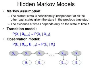
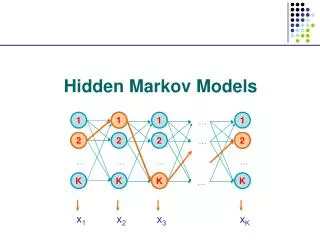
Discrete time finite Markov Chain Possible states: finite discrete set S {E1, E2, … … , Es} From time t to t+1, make stochastic movement from one state to another The Markov Property: At time t, the process is at Ej, Then at time t+1, the probability it is at Ek only depends on Ej The temporally homogeneous transition probabilities property: Prob(Ej→Ek) is independent of time t.
Discrete time finite Markov Chain • The transition probability matrix: • Pij=Prob(Ei→Ej) • An N step transition: Pij(N)=Prob(Ei→……. →Ejin N steps) • It can be shown that
Discrete time finite Markov Chain • Consider the two step transition probability from Ei to Ej: • This is the ijth element of • So, the two-step transition matrix • Extending this argument, we have • ---------------------------------------------------------------------------- • Absorbing states: • pii=1. Once enter this state, stay in this state. • We don’t consider this.
Discrete time finite Markov Chain The stationary state: The probability of being at each state stays constant. is the stationary state. For finite, aperiodic, irreducible Markov chains, exists and is unique. Periodic: if a state can only be returned to at t0, 2t0, 3t0,…….. , t0>1 Irreducible: any state can be eventually reached from any state
Discrete time finite Markov Chain Note: Markov chain is an elegant model in many situations in bioinformatics, e.g. evolutionary process, sequence analysis etc. BUT the two Markov assumptions may not hold true.
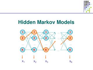
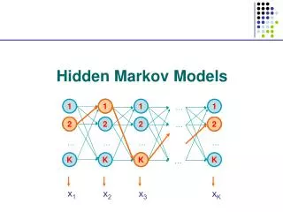
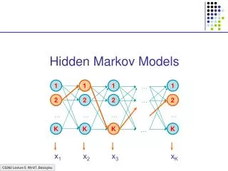
Hidden Markov Model More general than Markov model. A discrete time Markov Model with extra features. A Markov Chain Emission E1 O1 Initiation E2 O2 E3
Hidden Markov Model The emissions are probablistic, state-dependent and time-independent Example: 0.5 A B E1 E2 0.5 We don’t observe the states of the Markov Chain, but we observe the emissions. If both E1 and E2 have the same chance to initiate the chain, and we observe sequence “BBB”, what is the most likely state sequence that the chain went through? 0.1 0.8 0.25 0.75
Hidden Markov Model Let Q denote the state sequence, and O denote the observed emission. Our goal is to find: O=“BBB”, E1->E1->E1: 0.5*0.9*0.9*0.5*0.5*0.5= 0.050625 E1->E1->E2: 0.5*0.9*0.1*0.5*0.5*0.75= 0.0084375 E1->E2->E1: 0.5*0.1*0.8*0.5*0.75*0.5= 0.0075 E1->E2->E2: 0.5*0.1*0.2*0.5*0.75*0.75= 0.0028125 E2->E1->E1: 0.5*0.8*0.9*0.75*0.5*0.5= 0.0675 E2->E1->E2: 0.5*0.8*0.1*0.75*0.5*0.75= 0.01125 E2->E2->E1: 0.5*0.2*0.8*0.75*0.75*0.5= 0.0225 E2->E2->E2: 0.5*0.2*0.2*0.75*0.75*0.75= 0.0084375
Hidden Markov Model Parameters: initial distribution transition probabilities emission probabilities Common questions: How to efficiently calculate emissions: How to find the most likely hidden state: How to find the most likely parameters:
Hidden Markov Models in Bioinformatics A generative model for multiple sequence alignment.
Hidden Markov Models in Bioinformatics Data segmentation in array-based copy number analysis. R package aCGH in Bioconductor.
Hidden Markov Models in Bioinformatics An over-simplified model. Amplified Normal Deleted
The Forward and Backward Algorithm If there are a total of S states, and we study an emision from T steps of the chain, then #(all possible Q)=ST When either S or T is big, direct calculation is impossible. Let Let denote the hidden state at time t, Let bi denote the emission probabilities from state Ei Consider the “forward variables”: Emissions up to step t chain at state i at step t
The Forward and Backward Algorithm At step 1: At step t+1: … … … By induction, we know all Then P(O) can be found by A total of 2TS2computations are needed.
The Forward and Backward Algorithm Back to our simple example, find P(“BBB”) Now. What saved us the computing time? It is the reusing the shared components. And what allowed us to do that?. The short memory of the Markov Chain.
The Forward and Backward Algorithm The backward algorithm: From T-1 to 1, we can iteratively calculate: Emissions after step t chain at state i at step t
The Forward and Backward Algorithm Back to our simple example, observing “BBB”, we have
The Viterbi Algorithm To find: So, to maximize the conditional probability, we can simply maximize the joint probability. Define:
The Viterbi Algorithm Then our goal becomes: So, this problem is solved by dynamic programming.
The Viterbi Algorithm Time: 1 2 3 States: E1 0.5*0.5 0.15 0.0675 E2 0.5*0.75 0.05625 0.01125 The calculation is from left border to right border, while in the sequence alignment, it is from upper-left corner to the right and lower borders. Again, why is this efficient calculation possible? The short memory of the Markov Chain!
The Estimation of parameters When the topology of an HMM is known, how do we find the initial distribution, the transition probabilities and the emission probabilities, from a set of emitted sequences? Difficulties: Usually the number of parameters is not small. Even the simple chain in our example has 5 parameters. Normally the landscape of the likelihood function is bumpy. Finding the global optimum is hard.
The Estimation of parameters • The general idea of the Baun-Welch method: • Start with some initial values • Re-estimate the parameters • The previously mentioned forward- and backward-probabilities will be used. • It is guaranteed that the likelihood of the data improves with the re-estimation • Repeat (2) until a local optimum is reached • We will discuss the details next time. To be continued