Download
1 / 37
370 likes | 524 Vues
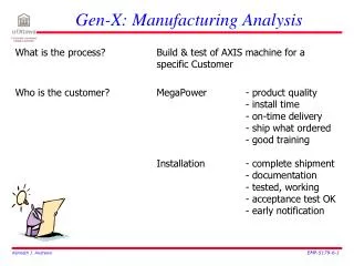
Gen-X: Manufacturing Analysis. What is the process? Build & test of AXIS machine for a specific Customer

E N D
Gen-X: Manufacturing Analysis What is the process? Build & test of AXIS machine for a specific Customer Who is the customer? MegaPower - product quality - install time - on-time delivery - ship what ordered - good trainingInstallation - complete shipment - documentation - tested, working - acceptance test OK - early notification
Gen-X: Manufacturing Analysis – Flowchart (1) • Order is logged in • Scheduled by the Manufacturing Manager (remote board) • Order sent to Manufacturing Engineer • Wait for drawings – always 5 days late • Initiate system build (before designs arrive) • Designs are checked, mistakes noted – no direct feedback • Problems with designs – try to reach designer WAIT • Mfg. Engineer modifies the designs (inventory-driven) • Supervisor takes the new designs • Systems are re-worked to account for actual designs • Parts are requested from Stores WAIT • Problems during build Mfg. Eng Mfg. Mgr Eng. Mgr • System hardware completed • System moved to Test
Gen-X: Manufacturing Analysis – Flowchart (2) • Chase software from Design WAIT • Software arrives (late) • Hardware functional check – problems fixed – no feedback • Software check – patches for bugs – documentation? • No time for Acceptance Test • System moved to shipping dock • Install Coordinator advised about imminent ship
Process Improvement What process? Improvements toa) fix root causes b) meet C requirements Customer +requirements Metrics (1-3 months) Map currentprocess Communicate plan Identifyhot-spots Implement,measure,fine-tune Root-causeanalysis
Manufacturing Systems: EMP-5179Module #6: Manufacturing Metrics Dr. Ken Andrews High Impact Facilitation Fall 2010
EMP-5179: Module #6 • Sigma, Variance, SPC etc. Revisited • Factory Physics • Balanced Scorecard
Even very rare outcomes are possible (probability > 0) Even very rare outcomes are possible (probability > 0) Fewer in the “tails” (upper) Fewer in the “tails” (lower) Most outcomes occur in the middle Variability The world tends to be bell-shaped
Process variability is determined byUS Mean Number of Samples Process Spread/Variability
Specification tolerance is defined by the Customer Mean Upper Specification Limit (USL) Lower Specification Limit (LSL) Number of Samples Specification Tolerance
Process Capability Indices We can be much more specific about process capability by measuring the process variability and comparing it directly to the required tolerance. Common measures are called Process Capability Indices (PCIs) μ= mean σ= std. deviation USL= Upper Spec. Limit LSL= Lower Spec. Limit
Process Capability USL – μ 3σ 24 – 20 3(2) = .667 = Cpk = min μ - LSL 3σ 20 – 15 3(2) = .833 = 15 24 14 20 26
Cpk measures “Process Capability” Good quality:defects are rare (Cpk>1) μ target
Cpk measures “Process Capability” If process limits and control limits are at the same location, Cpk = 1Cpk≥ 2 is exceptional. μ target Poor quality: defects are common (Cpk<1)
EMP-5179: Module #6 • Sigma, Variance, SPC etc. Revisited • Factory Physics • Balanced Scorecard
Factory Dynamics: Batch Production Consider a simple 4-station production line, where the processing time at each station is exactly 1 minute
Factory Dynamics: Single-Piece Flow Consider a simple 4-station production line, where the processing time at each station is exactly 1 minute
“Decrease Inventories” A factor of variability Lower WIP = Less Throughput = Not Good
“Reduce Variability AND Inventories” Reduced variability Lower WIP + Reduced variability = Higher Throughput = Good
Self-Paced Study Review and research the following material relating to: SCV Availability Factory Physics Confirm your understanding by following the examples provided.
Objective Measure of Variability For example, an assembly operation with an average process timeof 20 minutes and a standard deviation of 1 minute:scv = (1/20) 2 = 0.0025
Availability Consider a workstation that operates an average of 70 hoursbefore it must be shut down for maintenance, lasting 10 hours.
Optimal Maintenance Intervals? Infrequent maintenance:70 hours on, 10 hours off Frequent maintenance:3.5 hours on, 0.5 hours off What about variability? Isn’t that important too?
0.028 Optimal Maintenance Intervals?
Optimal Maintenance Intervals? scv = squared coefficient of variationmr = mean time to repairA = availabilityt0 = original processing time
Optimal Maintenance Intervals? Infrequent maintenance: 70 hours on, 10 hours off Frequent maintenance: 3.5 hours on, 0.5 hours off For the same equipment availability,shorter repair times lead to lower variabilityi.e. they are better
Utilization: High or Low? • One way to improve Return on Investment (ROI) is to maximize the revenue generated by utilizing production resources to the fullest extent possible = high capacity utilization. • Is a 24/7/52 factory a good strategy? • It depends on whether you are striving for shorter cycle times • It also depends on whether you are living in a:deterministic (ideal) world = very low variabilitystochastic (real) world = moderate/high variability
Cycle Time, Utilization & Variability CycleTime High Variability ModerateVariability Low Variability 20% 50% 100% Capacity Utilization Standard & Davis: “Running Today’s Factory”
Causes of Variability • Equipment downtime • Excessive set-up time • Uneven production demand • Batch material movement • Non-standard processes • Human factors • Supplier problems • Unexpected outages (e.g. power) • Reduce variability wherever possible throughout the production process. • Do not strive for 100% capacity utilization.
Preparation for Next Week • Watch for new articles/links on the website • Download material for module #7