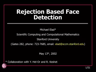
Rejection Based Face Detection
660 likes | 836 Vues
Rejection Based Face Detection. Michael Elad* Scientific Computing and Computational Mathematics Stanford University (Gates 282, phone: 723-7685, email: elad@sccm.stanford.edu ) May 13 th , 2002. * Collaboration with Y. Hel-Or and R. Keshet. Chapter 1 Problem Definition. Face Finder.

Rejection Based Face Detection
E N D
Presentation Transcript
Rejection Based Face Detection Michael Elad* Scientific Computing and Computational Mathematics Stanford University (Gates 282, phone: 723-7685, email: elad@sccm.stanford.edu) May 13th, 2002 * Collaboration with Y. Hel-Or and R. Keshet
Face Finder 1.1 Requirements Detect FRONTAL & VERTICAL faces: All spatial position, all scales any person, any expression Robust to illumination conditions Old/young, man/woman, hair, glasses. Design Goals: Fast algorithm Accurate (False alarms/ mis-detections)
1.2 Face Examples Taken from the ORL Database
Suspected Face Positions Input Image Compose a pyramid with 1:f resolution ratio (f=1.2) Draw L*L blocks from each location Classifier and in each resolution layer Face Finder 1.3 Position & Scale
1.4 Classifier? The classifier gets blocks of fixed size L2 (say 152) pixels, and returns a decision (Face/Non-Face) Block of pixels HOW ? Decision
Example: For blocks of 4 pixels Z=[z1,z2,z3,z4], we can assume that C(Z) is obtained by C(Z, θ)=sign{θ0 +z1 θ1+ z2 θ2+ z3 θ3+ z4 θ4} 2.1 Definition A classifier is a parametric (J parameters) function C(Z,θ) of the form
2.2 Classifier Design In order to get a good quality classifier, we have to answer two questions: • What parametric form to use? Linear or non-linear? What kind of non-linear? Etc. • Having chosen the parametric form, how do we find appropriate θ ?
2.3 Complexity Searching faces in a given scale, for a 1000 by 2000 pixels image, the classifier is applied 2e6 times THE ALGORITHMS’ COMPLEXITY IS GOVERNED BY THE CLASSIFIER PARAMETRIC FORM
2.4 Examples Collect examples of Faces and Non-Faces Obviously, we should have NX<<NY
2.5 Training The basic idea is to find θ such that or with few errors only, and with good GENERALIZATION ERROR
2.6 Geometric View C(Z,θ) is to drawing a separating manifold between the two classes +1 -1
3.1 Linear Separation The Separating manifold is a Hyper-plane +1 -1
3.2 Projection Projecting every block in this image onto a kernel is a CONVOLUTION
θ0 Mis- Detection False Alarm θ0 3.3 Linear Operation
Assume that and Gaussians Minimize variances Maximize mean difference *FLD - Fisher Linear Discriminant 3.4 FLD*
Maximize Minimize 3.6 FLD Formally
Generalized Eigenvalue Problem: Rv=Qv The solution is the eigenvector which corresponds to the largest eigenvalue 3.7 Solution Maximize
3.8 SVM* Among the many possible solutions, choose the one which Maximizes the minimal distance to the two example-sets *SVM - Support Vector Machine
3.9 Support Vectors 1. The optimal θ turns out to emerge as the solution of a Quadratic-Programming problem 2. The support vectors are those realizing the minimal distance. Those vectors define the decision function
3.10 Drawback Linear methods are not suitable 1. Generalize to non-linear Discriminator by either mapping into higher dimensional space, or using kernel functions 2. Apply complex pre-processing on the block Complicated Classifier!!
3.11 Previous Work • Rowley & Kanade (1998), Juel & March (96): • Neural Network approach - NL • Sung & Poggio (1998): • Clustering into sub-groups, and RBF - NL • Osuna, Freund, & Girosi (1997): • Support Vector Machine & Kernel functions - NL • Osdachi, Gotsman & Keren (2001): • Anti-Faces method - particular case of our work • Viola & Jones (2001): • Similar to us (rejection, simplified linear class., features)
4.1 Model Assumption Faces Non-Faces We think of the non-faces as a much richer set and more probable, which may even surround the faces set
Projected onto θ 1 Rejected points 4.2 Maximal Rejection Find θ1 and two decision levels such that the number of rejected non-faces is maximized while finding all faces
Rejected points Projected onto θ 2 4.3 Iterations Taking ONLY the remaining non-faces: Find θ2 and two decision levels such that the number of rejected non-faces is maximized while finding all faces Projected onto θ 1 Shree Nayar & Simon Baker (95) - Rejection
4.4 Formal Derivation Maximal Rejection Maximal distance between these two PDF’s We need a measure for this distance which will be appropriate and easy to use
Maximize the following function: Maximize the distance between all the pairs of [face, non-face] A Reighly Quotient Minimize the distance between all the pairs of [face, face] 4.5 Design Goal
4.6 Objective Function • The expression we got finds the optimal kernel θ in terms of the 1st and the 2nd moments only. • The solution effectively project all the X examples to a near-constant value, while spreading the Y’s away - θ plays a role of an approximated invariant of the faces • As in the FLD, the solution is obtained problem is a Generalized Eigenvalue Problem.
5.1 General There are two phases to the algorithm: 1. Training:Computing the projection kernels, and their thresholds. This process is done ONCE and off line 2. Testing: Given an image, finding faces in it using the above found kernels and thresholds.
Compute Remove Minimize f(θ) & find thresholds Compute Sub-set END 5.2 Training Stage
No more Kernels Face Project onto the next Kernel Is value in Non Face No Yes 5.3 Testing Stage
178 false-alarms 136 false-alarms 3 1 875 false-alarms 5 37 false-alarms 6 66 false-alarms 4 35 false-alarms 2 5.5 2D Example Original yellow set contains 10000 points
5.6 Limitations • The discriminated zone is a parallelogram. Thus, if the faces set is non-convex, zero false alarm is impossible!! Solution: Second Layer • Even if the faces-set is convex, convergence to zero false-alarms is not guaranteed. Solution: Clustering
- We are dealing with frontal and vertical faces only • - We are dealing with a low-resolution representation of the faces 5.7 Convexity? Can we assume that the Faces set is convex?
Chapter 6 Pre-Processing No time ? Press here
6.1 Pre-Process Typically, pre-processing is an operation that is done to each block Z before applying the classifier, in order to improve performance Face/Non-Face Pre-Processing Z Classifier Problem: Additional computations !!
6.2 Why Pre-Process Example: Assume that we would like our detection algorithm to be robust to the illumination conditions system Option: Acquire many faces with varying types of illuminations, and use these in order to train the system Alternative: Remove (somehow) the effect of the varying illumination, prior to the application of the detection algorithm – Pre-process!
6.3 Linear Pre-Process If the pre-processing is linear (P·Z): The pre-processing is performed on the Kernels ONCE, before the testing !!
6.4 Possibilities 1. Masking to disregard irrelevant pixels. 2. Subtracting the mean to remove sensitivity to brightness changes. Can do more complex things, such as masking some of the DCT coefficients, which results with reducing sensitivity to lighting conditions, noise, and more ...
7.1 Details • Kernels for finding faces (15·15) and eyes (7·15). • Searching for eyes and faces sequentially - very efficient! • Face DB: 204 images of 40 people (ORL-DB after some screening). Each image is also rotated 5 and vertically flipped - to produce 1224 Face images. • Non-Face DB: 54 images - All the possible positions in all resolution layers and vertically flipped - about 40·106 non-face images. • Core MRC applied (no fancy improvements).
7.2 Results - 1 Out of 44 faces, 10 faces are undetected, and 1 false alarm (the undetected faces are circled - they are either rotated or shadowed)
7.3 Results - 2 All faces detected with no false alarms
7.4 Results - 3 All faces detected with 1 false alarm (looking closer, this false alarm can be considered as face)
7.5 Complexity • A set of 15 kernels - the first typically removes about 90% of the pixels from further consideration. Other kernels give a rejection of 50%. • The algorithm requires slightly more that oneconvolution of the image (per each resolution layer). • Compared to state-of-the-art results: • Accuracy – Similar to (slightly inferior in FA) to Rowley and Viola. • Speed – Similar to Viola – much faster (factor of ~10) compared to Rowley.