Rejection Based Face Detection
Rejection Based Face Detection. Michael Elad* Scientific Computing and Computational Mathematics Stanford University The Computer Vision Workshop March 18 th , 2002. * Collaboration with Y. Hel-Or and R. Keshet. Part 1 Introduction of the Problem and Basic Considerations. Part 1.

Rejection Based Face Detection
E N D
Presentation Transcript
Rejection Based Face Detection Michael Elad* Scientific Computing and Computational Mathematics Stanford University The Computer Vision Workshop March 18th, 2002 * Collaboration with Y. Hel-Or and R. Keshet
Part 1 1. The Task Input image Face (target) Detector • Comments: • Extension to color • Faces vs. general targets
Part 1 2. Requirements • Detect frontal & vertical faces: • All spatial position, all scales • Any person, any expression • Robust to illumination conditions • Old/young, man/woman, hair, glasses. • Design Goals: • Fast algorithm • Accurate (False Positive / False Negative)
Part 1 3. Frontal-Vertical Faces Taken from the ORL Database
Face Finder Part 1 4. Scale-Position Input Image Suspected Face Positions Compose a pyramid with 1:f resolution ratio (f=1.2) Draw L*L blocks from each location Classifier and in each resolution layer
Need to answer two questions: Q1: What parametric form to use? Linear or non-linear? What kind of non-linear? Etc. Q2: Having chosen the parametric form, how do we find appropriate set of parameters θ ? Part 1 5. Classifier Design A classifier is a parametric (J parameters) function C(Z,θ) of the form
Part 1 6. Algorithm Complexity Searching faces in a given scale, for a 1000 by 2000 pixels image, the classifier is applied 2e6 times (Q1) Choosing the parametric form: keep in mind that the algorithm’s complexity is governed by the classifier complexity
(Q2) Finding Suitable Parameters: Part 1 7. Training by Examples
Part 1 8. Geometric Interpretation C(Z,θ) is to drawing a separating manifold between the two classes +1 -1
Part 2 1. Neural Networks • Choose C(Z,θ) to be a Neural Network (NN). • Add prior knowledge in order to: • Control the structure of the net, • Choose the proper kind (RBF ?), • Pre-condition the data (clustering) • Representative Previous Work: • Juel & March (1996), and • Rowley & Kanade (1998), and • Sung & Poggio (1998). NN leads to a Complex Classifier
Part 2 2. Support Vector Machine • Choose C(Z,θ) to be a based on SVM. • Add prior knowledge in order to: • Prune the support vectors, • Choose the proper kind (RBF, Polynomial ?), • Pre-condition the data (clustering) • Representative Previous Work: • Osuna, Freund, & Girosi (1997), • Bassiou et.al.(1998), • Terrillon et. al. (2000). SVM leads to a Complex Classifier
Part 2 3. Rejection Based • Build C(Z,θ) as a combination of weak (simple to design and activate) classifiers. • Apply the weak classifiers sequentially while rejecting non-faces. • Representative Previous Work: • Rowley & Kanade (1998) • Elad, Hel-Or, & Keshet (1998), • Amit, Geman & Jedyank (1998), • Osdachi, Gotsman & Keren (2001), and • Viola & Jones (2001). Fast (and accurate) classifier
Input Blocks Rejected Rejected Weak Classifier # n Weak Classifier # 2 Weak Classifier # 3 Weak Classifier # 4 Weak Classifier # 1 Detected … Rejected Rejected Rejected Part 2 4. The Rejection Idea Classifier
Part 2 5. Supporting Theory • (Ada) Boosting – Freund & Schapire (1990-2000) – Using a group of weak classifiers in order to design a successful complex classifier. • Decision-Tree – Tree structured classification (the rejection approach here is a simple dyadic tree). • Rejection – Nayar & Baker (1995) - Application of rejection while applying the sequence of weak classifiers. • Maximal Rejection – Elad, Hel-Or & Keshet (1998) – Greedy approach towards rejection.
+1 -1 Hyperplane Part 3 1. Linear Classification (LC) We propose LC as our weak classifier:
Projected onto θ 1 Rejected non-faces Part 3 2. Maximal Rejection Find θ1 and two decision levels such that the number of rejected non-faces is maximized while finding all faces Non-Faces Faces
Rejected points Projected onto θ 2 Part 3 3. Iterations Taking ONLY the remaining non-faces: Find θ2 and two decision levels such that the number of rejected non-faces is maximized while finding all faces Projected onto θ 1
Part 3 4. Maximizing Rejection Maximal Rejection Maximal distance between these two PDF’s We need a measure for this distance which will be appropriate and easy to use
Part 3 5. One Sided Distance Define a distance between a point and a PDF by This distance is asymmetric !! It describes the average distance between points of Y to the X-PDF, PX().
In the case of face detection in images we have P(X)<<P(Y) We Should Maximize (GEP) Part 3 6. Final Measure
Maximize the following function: Maximize the distance between all the pairs of [face, non-face] The same Expression Minimize the distance between all the pairs of [face, face] 7. Different Method 1
8. Different Method 2 If the two PDF’s are assumed Gaussians, their KL distance is given by And we get a similar expression
The discriminated zone is a parallelogram. Thus, if the faces set is non-convex*, zero false alarm discrimination is impossible – Solution: Second layer. * More accurately, if in the convex hull of the face set there are non-faces Part 3 9. Limitations • Even if the faces-set is convex, convergence to zero false-alarms is not guaranteed. – Solution: Clustering the non-faces.
- We are dealing with frontal and vertical faces only • - We are dealing with a low-resolution representation of the faces Part 3 8. Convexity? Can we assume that the Faces set is convex? • - Are they any non-faces that are convex combination of faces ?
Part 4 1. Details • Kernels for finding faces (15·15) and eyes (7·15). • Searching for eyes and faces sequentially - very efficient! • Face DB: 204 images of 40 people (ORL-DB after some screening). Each image is also rotated 5 and vertically flipped - to produce 1224 Face images. • Non-Face DB: 54 images - All the possible positions in all resolution layers and vertically flipped - about 40·106 non-face images. • Core MRC applied (no second layer, no clustering).
Part 4 2. Results - 1 Out of 44 faces, 10 faces are undetected, and 1 false alarm (the undetected faces are circled - they are either rotated or strongly shadowed)
Part 4 3. Results - 2 All faces detected with no false alarms
Part 4 4. Results - 3 All faces detected with 1 false alarm (looking closer, this false alarm can be considered as face)
Part 4 5. More Details • A set of 15 kernels - the first typically removes about 90% of the pixels from further consideration. Other kernels give a rejection of 50%. • The algorithm requires slightly more that oneconvolution of the image (per each resolution layer). • Compared to state-of-the-art results: • Accuracy – Similar to (slightly inferior in FA) to Rowley and Viola. • Speed – Similar to Viola – much faster (factor of ~10) compared to Rowley.
Part 4 6 .Conclusions • Rejection-based classification - effective and accurate. • Basic idea – group of weak classifiers applied sequentially followed each by rejection decision. • Theory – Boosting, Decision tree, Rejection based classification, and MRC. • The Maximal-Rejection Classification (MRC): • Fast – in close to one convolution we get face detection, • Simple – easy to train, apply, debug, maintain, and extend. • Modular – to match hardware/time constraints. • Limitations – Can be overcome. • More details – http://www-sccm.stanford.edu/~elad
7 . More Topics • Why scale-invariant measure? • How we got the final distance expression? • Relation of the MRC to Fisher Linear Discriminant • Structure of the algorithm • Number of convolutions per pixel • Using color • Extending to 2D rotated faces • Extension to 3D rotated faces • Relevancy to target detection • Additional ingredients for better performance
Same distance for 1. Scale-Invariant
In this expression: • The two classes means are encouraged to get far from each other • The Y-class is encouraged to spread as much as possible, and • The X-class is encouraged to condense to a near-constant value • Thus, getting good rejection performance. back
Minimize variances Maximize mean difference 3. Relation to FLD* Assume that and Gaussians *FLD - Fisher Linear Discriminant
Maximize Minimize
In the MRC we got the expression for the distance If P(X)=P(Y)=0.5 we maximize The distance of the X points to the Y-distribution The distance of the Y points to the X-distribution
Instead of maximizing the sum Minimize the inverse of the two expressions (the inverse represent the proximity) back
Compute Remove Minimize f(θ) & find thresholds Compute Sub-set END 4. Algorithm Structure
No more Kernels Face Project onto the next Kernel Is value in Non Face No Yes back
5. Counting Convolutions • Assume that the first kernel rejection is 0<<1 (I.e. of the incoming blocks are rejected). • Assume also that the other stages rejection rate is 0.5. • Then, the number of overall convolutions per pixel is given by back
6. Using Color • Several options: • Trivial approach – use the same algorithm with blocks of L-by-L by 3. • Exploit color redundancy – work in HSV space with decimated versions of the Hue and the Saturation layers. • Rejection approach – Design a (possibly non-spatial) color-based simple classifier and use it as the first stage rejection. back