Download
1 / 31
310 likes | 334 Vues
This study explores the intricate many-electron effects in molecular quantum dots, focusing on Coulomb blockade phenomena and their impact on transport behavior. The research delves into understanding the intricate interactions between electron levels, filled and empty states, and charging effects within the system.

E N D
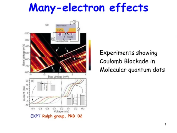
Many-electron effects EXPTRalph group, PRB ‘02 Experiments showing Coulomb Blockade in Molecular quantum dots
So far we’ve seen • Transport is determined by a few levels near EF • These levels are broadened by the contacts and shifted by the local potential • The levels come from solving Schrodinger Equation for the channel. For individual atoms, this is done self- consistently with an approximate el-el interaction • Atomic levels combine to form molecular levels stabilized by long-ranged electrostatic forces (ionic bonds) or short-ranged quantum forces (covalent bonds)
µ2 + Broadening D(E) + Electrostatics U (Self-consistent Field) g1 g2 µ1 SOURCE DRAIN CHANNEL INSULATOR VG VD I Minimal Model for Transport Rate equation g1,2, f1,2 Levels obtained by solving one-electron Schrodinger equation with approximate el-el interaction
Can we do better than that? Suppose we have a computer big enough to solve the many-electron Schrodinger equation. How would we use those results?
1 level Many el ‘levels’ Total Energy EN Probability ‘1’ P1 e0 P0 0 ‘0’ One Electron ‘level’ e0 “Fock” Space
e0 + U e0 2 levels Total Energy EN Probability “11” P11 2e0 + U “10” “01” e0 P01, 10 0 P00 “00”
Equilibrium occupancy Many el ‘levels’ Total Energy EN Probability ‘1’ P1 e0 P0 0 ‘0’ P1 = e-(e0-m)/[1+e-(e0-m)] = f(e0) P0 = 1/[1+e-(e0-m)] = 1-f(e0) One Electron ‘level’ e0 PN = e-(EN-mN)/kT/Z, Z = SN e-(EN-mN)/kT
Equilibrium occupancy Many el ‘levels’ Total Energy EN Probability ‘1’ P1 e0 P0 0 ‘0’ P1 = e-(e0-m)/[1+e-(e0-m)] = f(e0) P0 = 1/[1+e-(e0-m)] = 1-f(e0) One Electron ‘level’ e0 <N> = 0.P0 + 1.P1 = f(e0)
Equilibrium occupancy gf/ħ g(1-f)/ħ dP0/dt = -gfP0/ħ + g(1-f)P1/ħ gfP0/ħ - g(1-f)P1/ħ dP1/dt = ‘1’ ‘0’ P0 + P1 = 1 P1 = e-(e0-m)/[1+e-(e0-m)] = f(e0) Ratio = e-(e0-m)/kT P0 = 1/[1+e-(e0-m)] = 1-f(e0)
2 levels Total Energy EN U ∞ e0 0 P00 = 1/Z P01 = P10 = e-(e0-m)/kT/Z Z = 1 + 2e-(e0-m)/kT <N> = 0.P00 + 1.(P01+ P 10) = 1/[1+ ½e(e0-m)/kT]
Now what happens under Nonequilibrium? Contacts create transitions between these many-electron levels
Transition rates between the states g1f1/ħ + g2f2/ħ g1(1-f1)/ħ + g2(1-f2)/ħ Rate of adding an electron Rate of removing an electron (g1f1+ g2f2)P0/ħ [g1(1-f1)+g2(1-f2)]P1/ħ ‘1’ ‘0’
Rate equations in many-el space g1f1/ħ + g2f2/ħ g1(1-f1)/ħ + g2(1-f2)/ħ ‘1’ ‘0’ dP0/dt = -(g1f1+ g2f2)P0/ħ + [g1(1-f1) + g2(1-f2)]P1/ħ dP1/dt = (g1f1+ g2f2)P0/ħ - [g1(1-f1) + g2(1-f2)]P1/ħ P0 + P1 = 1
Solution g1f1+ g2f2 g1f1+ g2f2 g1+ g2 g1+ g2 [g1(1-f1)+ g2(1-f2)] g1+ g2 <N> = P0.0 + P1.1 = g1f1 P0 –g1(1-f1)P1 g1g2 (f1-f2) I1 = q = q ħ (g1 + g2) P1 = P0 = ħ
g1f1/ħ + g2f2/ħ g1(1-f1)/ħ + g2(1-f2)/ħ g1f1+ g2f2 <N> = g1(1+f1) + g2(1+f2) 2 levels Total Energy EN U ∞ e0 0 dP00/dt = ... dP01/dt = ... ...
What did we achieve? We can now write down rate equations in one electron space with approximate el-el interactions (SCF) OR rate equations directly in many-electron configuration space with exact el-el interactions • What is the relation between the two descriptions? • When do we use which?
Relation between many-el and one-el levels Filled levels represent Ionization energy: Energy to take electron from the single N electron Ground state to one of the multiple (N-1) electron states IP(n) = EN(0) – EN-1(n)
Ionization Energies 1st IP E4(0) – E3(0) 2nd IP 3 el GS E3(0) 3 el Excited St E3(1) 3rd IP 4th IP E3(3) E3(2) 4 el Ground state E4(0)
Ionization Energies 1st IP E4(0) – E3(0) 2nd IP 3 el GS E3(0) 3 el Excited St E3(1) 3rd IP 4th IP E3(3) E3(2) Ionization Levels
What do empty energies mean? Empty levels represent Electron Affinity: Energy to add an electron to N electron ground state to create one of the multiple (N+1) electron states EA(n) = EN+1(n) – EN(0)
When do we need many-el viewpoint? When charging is important U0 >> (g1 + g2), kBT In the opposite limit, got by with U = UL + U0DN Many-el generalization, U0 Hartree term But this doesn’t suffice if U0 large
What does charging do? Uee(N) = U0N(N-1)/2 (U0 times # pairs) IP(n) = EN(0) – EN-1(n) = eHOMO + U0(N-1) EA(n) = EN+1(n) – EN(0) = eLUMO + U0N (extra charge due to extra el repulsion) Charging opens gap U0 between filled and empty levels But here we add charging contribution differently to different levels
eLUMO eLUMO U0/2 eLUMO eHOMO U0/2 eHOMO U0/2 eHOMO Bare levels in absence of charging Approx. level-independent wayto add charging Uscf(N) = ∂Uee/∂N = U0(N-1/2) Say N=1 at equilibrium Add charging through Uscf (shifts levels) Add charging exactly (increases gap) So to capture this with SCF, need to make the potential level-dependent
Does this affect the I-V? One might expect that the opening of the gap with U0 should make it harder to add a charge, giving an initial low conductance regime in the I-V (“Coulomb Blockade”) Would not notice this if g >> U0 How would our equations give this?
Configuration space for 2 spins Write down rate equations between all states The resulting I-V should give the correct answer (Homework)
I0 RSCF 2I0/3 Exact I0/2 USCF 11 10 01 00 Coulomb Blockade in I-V RSCF: U = U0(N-N0) USCF: U = U0(N-N0) U = U0(N-N0)
Expt (Ralph group) Theory (PRB ’06) Expt (Zhitenev group) Theory (unpublished) BANIN et al, Nature ‘99 Experiments a bit more complex
If trapped charge cannot escape, hysteresis Consistent with expts from UVA Trap Channel Drain Source CB between ‘trap’ and channel
Molecular Coulomb Blockade (Zhitenev) Molecular Kondo (Ralph/McEuen) When Electrons Cooperate (“Correlation”) Magnets, superconductors (A + B)(A + B) (AB - AB)
Summary For small charging, usual method of writing rate equations in real space work. Use Schrodinger equation with approximate SCF potential U and broadening to get currents. For large charging, SCF is not enough. Would need to work with rate equations in full many-electron configuration space with exact el-el interactions included. This would give Coulomb Blockade. Trouble with the latter • Size of conf. space increases fast (2N for N orbitals) • Don’t know how to broaden the levels or the transitions
What next? Let’s go back now to the SCF approach to transport, keeping in mind that the approach need to be modified for large charging and Coulomb Blockade. We now understand what the SCF ‘levels’ represent, ie, ionization energies/electron affinities that represent transitions between many-electron levels. We know how to calculate the SCF levels for atoms and molecules, the latter forming covalent bonds on occasion. We’ll next see how these bonds can extend in a solid to form bands