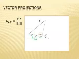
VecTOR PROJECTionS
VecTOR PROJECTionS. 90˚. Matrix Operation: Inverse MAtrix. Important for solving a set of linear equations, is the matrix operation that d efines an inverse of a matrix. X -1 : Inverse matrix of X. X -1 X = I

VecTOR PROJECTionS
E N D
Presentation Transcript
Matrix Operation: Inverse MAtrix Important for solving a set of linear equations, is the matrix operation that defines an inverse of a matrix. X-1 : Inverse matrix of X X-1 X = I where I is the identity matrix:all entries on the diagonal are 1,all others 0 ( here for 3 x 3 matrix)
Matrix Operation: Important for solving a set of linear equations, is the matrix operation that defines an inverse of a matrix. X-1 : Inverse matrix of X X-1 X = Iwhere I is the identity matrix Not all matrices have an inverse matrix and there is not a simple rule how to calculate the entries in an inverse matrix! We skip the formal mathematical aspects and note here only the important facts: For symmetric square matrices like covariance matrices or correlation matrices the inverse exists
Summary Simple Linear Regression Principal Component Analysis
Summary 2-dimensional sample space: Simple Linear Regression: Minimizes the Summed Squared Errors (measured in the vertical direction between Fitted regression line and observed data points) Principal Component Analysis: Finds the direction of vector that maximizes the variance that is projecting onto this vector.
Regression analysis in R Simple linear regression in R: the function res<-lm( y ~ x ) calculates the linear regression line It returns a number of useful additional statistical measures of the quality of the regression line.
Residuals (errors) res$residuals Remember: We assumed that errorsare uncorrelated to the ‘predictor’ variable x. It is recommended to check that the errors itself do NOT have an organized structure when plotted over x.
Histogram of residuals (errors) hist(res$residuals) Remember: We assumed that errorsare uncorrelated to the ‘predictor’ variable x. It is recommended to check also if the errors follow a Gaussian (bell-shaped) distribution. Note: the function fgauss() is defined in myfunctions.R [call source(“scripts/myfunctions.R”)]
Linear Regression statistics When applying linear regression, a number of test statistics are calculated in R’s lm() function. Slope of regression line Statistical significance: The smaller thevalue, the higher the significance of the linear relationship (slope >0) Regression Parameter (slope) Correlation coefficient between the fitted y-values and observed y-values
Linear Regression:usE the Linear Regression with caution! Outliers can have a large effect and suggest a linear relationship where there is none! It can be tested for the influence of single outlier observations. The sample space is important! If you only observed x and y in a limited range or a subdomain of the sample space,
Linear Regression:The Danger of using the Linear Regression! Outliers can have a large effect and suggest a linear relationship where there is none! It can be tested for the influence of single outlier observations. The sample space is important! If you only observed x and y in a limited range or a subdomain of the sample space, extrapolation can give misleading results
Multiple LINEAR REGRESSION Random Error (noise) Predictand (e.g. Albany Airport Temperature anomalies) Predictors: e.g.: Temperatures from nearby stations or: Indices of Large-Scale Climate Modeslike El Nino Southern Oscillation, North Atlantic Oscillation or: prescribed time-dependent functions like linear trend, periodic oscillation, polynoms Source: http://reliawiki.org/index.php/Multiple_Linear_Regression_Analysis (figures retrieved April 2014)
Multiple LINEAR REGRESSION Write a set of linear equations for each observation in the sample (e.g. for each year of temperature observations Source: http://reliawiki.org/index.php/Multiple_Linear_Regression_Analysis (figures retrieved April 2014)
Multiple LINEAR REGRESSION Or in short Matrix notation Source: http://reliawiki.org/index.php/Multiple_Linear_Regression_Analysis (figures retrieved April 2014)
Multiple LINEAR REGRESSION size of the vectors / matrices: n x 1 n x k k x 1 n x 1 The mathematical problem we need to solve is: Given all the observations of the predictand (stored in vector ) and the predictor variables stored in matrix X, we want to find simultaneously a for each predictor variable a proper scaling factor, such that the fitted estimated values minimize the sum of the squared errors. Source: http://reliawiki.org/index.php/Multiple_Linear_Regression_Analysis (figures retrieved April 2014)
Multiple LINEAR REGRESSION We find here the covariance matrix (scaled by n) of the predictor variables. The ‘-1’ indicates another fundamentally important matrix operation: The inverse of a matrix Covariance (scaled by n) of all predictors with the predictand size of the vectors / matrices: k x 1 ( k x n n x k ) k x n n x 1 (k x k) (k x 1) Source: http://reliawiki.org/index.php/Multiple_Linear_Regression_Analysis (figures retrieved April 2014)
Multiple LINEAR REGRESSION The resulting kx1 matrix (i.e. vector) contains a proper scaling factor for each predictor. In other words: multiple linear regression is a weighted sum of the predictors (after conversion intounits of the predictand y). size of the vectors / matrices: k x 1 ( k x n n x k ) k x n n x 1 (k x k) (kx1) Source: http://reliawiki.org/index.php/Multiple_Linear_Regression_Analysis (figures retrieved April 2014)
Example Multiple Linear Regressionwith 2 predictors The scatter cloud shows a linear dependence of the values in y along the two predictor dimensions x1 x2.
General rule: work with as few predictors as possible. (every time you add a new predictoryou increase the risk of over-fitting the model) Observe how good the fitted values and observed values match (correlation) Choose predictors that provide independent information about the predictand The problem of collinearity: If the predictors are all highly correlated among each otherthen the MLR can become very ambiguous (because it gets harder to calculate accurately the inverse of the covariance matrix) Last but not least: the regression coefficients from the MLR are not ‘unique’. If you add or remove one predictor, all regression coefficients can change. Tips for multiple linear regression (MLR)
Global Sea Surface Temperatures Principal Component Analysis From voluntary ship observations colors show the percentage of months with at least one observation in a 2 by 2 degree grid box. From paper in Annual Review of Marine Science (2010)
Global Sea Surface Temperatures Principal Component Analysis Climatology 1982-2008 Red areas mark regions with highest SST variability
Global Sea Surface Temperatures Principal Component Analysis Principal Component Analysis (PCA) (Empirical Orthogonal Functions (EOF)) The first leading Eigenvector Eigenvectors form now geographic pattern. Grids with high positive values and large negative values are covarying out of phase (negative correlation). Green regions show small variations in this Eigenvector #1. The Principal Component is a time series showing the temporal evolution of the SST variations. This mode is associated with the El Niño - Southern Oscillation