Solving 8-Puzzle Problem with Search Algorithms
Understand the application of search algorithms in solving the 8-puzzle problem, exploring BFS and DFS approaches, complexities, and implementations. Learn the significance of memory usage and time complexity.

Solving 8-Puzzle Problem with Search Algorithms
E N D
Presentation Transcript
GENERAL PROBLEM SOLVINGWITH SEARCH ALGORITHMS (C) Debasis Mitra
8-PUZZLE PROBLEM SOLVING Input: Goal: (C) Debasis Mitra
8-PUZZLE PROBLEM SOLVING Input: 2 possible moves: Goal (C) Debasis Mitra
8-PUZZLE PROBLEM SOLVING Input: Branching factor, b=2 b=3 b=3 3, D 6, U 5, R 5, U 2, R 1, L Goal (C) Debasis Mitra
Problem Solving = Graph Search • Search algorithm creates a Search Tree • Branching Factor may increase or decrease, for the above: 2, 3, 4 • Tree Search: Same pattern may be repeated! • That may mean looping • Really, Graph Search: use memory to remember visited nodes • Note, it is being <<dynamically>> performed: Generate-and-Test • Test in each iteration, if solution is reached • Search tree is dynamically getting generated during search (C) Debasis Mitra
Problem Solving = Graph Search • AI search: The Graph may NOT be statically available as input • Some input board may not have any solution! • Problem Solving in AI is often (always!): Graph Search • It is mostly graph search, but often we treat it as a tree search, • often ignoring, repeat of nodes because that would be too expensive to check! • Each node is a “state”: State space is searched • Breadth First Search (BFS) • Depth First Search (DFS) (C) Debasis Mitra
Sliding Puzzle Solving with BFS/DFS Input or Problem instance • Think of input data structure. • Input Size n= • 8-Puzzle: 3x3 tiles, n= 9 • 15-Puzzle: 4x4 tiles, n=16 • … • Problem Complexity= Total number of feasible steps over a search tree • What are the steps: Left/Right/Up/Down • Complexity as O(f(n)) • #Steps: O(bn), for average branching factor b: • Branching means, how many options available at each step Goal (C) Debasis Mitra
AI Problem Solving • NP-hard problems: likely to be O(kn), for some k>1, exponential • Clever, efficient algorithms exist, but worst case remains exponential • AI is often about efficiently solving by clever algorithm! (C) Debasis Mitra
BFS: 8-PUZZLE PROBLEM SOLVING Input: Black arrows show the structure of the tree Red arrows show control flow b=3 b=3 3, D 6, U 5, R 5, U 2, R 1, L Goal What is the typical data structure for BFS? Queue or Stack? (C) Debasis Mitra
Breadth First Search Algorithm BFS(s): s start node 0. Initialize a Q with s; • v = Pop(Q); // BFS is Queue based algorithm • If v is “goal” return success; • mark node v as visited; // configurations generated before, // not done in “tree” search mode 4. operate on v; // e.g., evaluate if it is the goal node, then return 5. for each node w accessible from node v do 6. if w is not marked as visited then // with generate-and-test this may not be time consuming 7. Push w at the back of Q; end for; End algorithm. Code it! (C) Debasis Mitra
DFS: 8-PUZZLE PROBLEM SOLVING Input: Red and green arrows are control flow b=3 b=3 3, D 6, U 5, R 5, U 2, R 1, L Until leaf node, no more children Goal (C) Debasis Mitra
Depth First Search Algorithm DFS(v)// recursive • mark node v as visited; // configurations generated before, // not done in “tree” search mode • If v is “goal” return success; • operate on v ; // e.g., evaluate if it is the goal node • for each node w accessible from node v do • if w is not marked as visited then// again, not done in “tree” search mode 6. DFS(w); // an iterative version of this //will maintain its own stack end for; End algorithm. Driver algorithm Input: Typical Graph search input is a Graph G: (nodes V, arcs E) // Here we have: a board as a node p, and operators for modifying board correctly // i.e, we generate the graph as we go: “Generate and Test” Output: Path to a goal node g, typically computer will display the next node on the path call DFS(p); // input board p as a node in search tree G End. (C) Debasis Mitra
BFS vs DFS • BFS: • Memory intensive: ALL children are to be stored from all levels • At least all nodes of the last level are to be stored, and that grows fast too! • Also, you cannot do above if the path from start node to goal is needed! • If goal exists, BFS is guaranteed to find it: complete algorithm • (systematically finds it, level by level) • If goal is nearby (at a low level), BFS quickly finds it • Memory intensive, all nodes in memory • Queue for implementation • DFS: • Infinite search is possible, in the worst case • May get stuck on an infinitedepth in a branch, • Even if the goal may be at a low level on a different branch • Linear memory growth, depth-wise WHY? • but, go to the point number 1 above memory may explode for large depth! • Stack for implementation (equivalent to recursive implementation) (C) Debasis Mitra
BFS vs DFS • Time complexity: Worst case for both, all nodes searched: O(bd) b branching factor, d depth of the goal • Memory: • BFS O(bd) remember all nodes • DFS O(bd), only one set of children at each level, up to goal depth • But the depth may be very high, up to infinity • DFS <forgets> previously explored branches Goal (C) Debasis Mitra
Depth Limited Search (DLS):To avoid infinite search of DFS • Stop DFS at a fixed depth l, no mater what • Goal, may NOT be found: Incomplete Algorithm • If goal depth d > l • Why DLS? To avoid getting stuck at infinite (read: large) depth • Time: O(bl), Memory: O(bl) Goal (C) Debasis Mitra
Iterative Deepening Search (IDS) • Repeatedly stop DFS at a fixed depth l (i.e., DLS), AND • If goal is not found, • then RESTART from start node again, with l = l+1 • Complete Algorithm • Goal <<will>> be found when l = = d, goal depth • Isn’t repetition very expensive? • Time: O(b1 +b2 +b3 + .. bd ) = O(bd+1), as opposed to O(bd), • For b=10, d=5, this is 111,000 to 123,450 increase , 11% • Memory: • IDS vs DFS: same O(bd) • IDS vs BFS: O(bd) vs O(bd) (C) Debasis Mitra
Informed Search (Heuristics Guided Search) (C) Debasis Mitra
Informed Search (Heuristics Guided Search, or “AI search”) • Available is a “heuristic” function f(n) node n, to chose a • best Child node from alternative nodes • Example: Guessed distance from goal • You can see the Eiffel tower (goal), move towards it! • Best_Child = Child w with minimumf(w) • We will use h(w) for node w as guessed distance to goal • AI-searches are optimization problems • Both BFS and DFS may be guided: Informed search (C) Debasis Mitra
Uniform Cost (Breadth First) Search Algorithm ucfs(v) • Enqueue start node s on a min-priority queue Q; // distance g(s)= 0 • While Q ≠ empty do 3. v = pop(Q); 4. If v is a goal return success; 5. Operate on v (e.g., display board); 6. For each child w of v, • Insert w in Q such that h(w) is the lowest; // h(w) is path cost from node w to a goal node, // replacing h(w) with g(w), distance of w from source, makes it Djikstra’s algorithm // Q is a priority-queue to keep lowest cost-node in front (C) Debasis Mitra
Uniform Cost Search: Breadth First with weights rather than levels Algorithm ucs(v) • Enqueue start node s on a min-priorityqueue Q; // distance h(s)= 0 • While Q ≠ empty do 3. v = pop(Q); // lowest path-cost node 4. If v == a goal return success; 5. operate on v (e.g., display board); 6. For each child w of v, if w is not-visited before, 7. Insert w in Q such that g(w) is the lowest; // use priority-que or heap for Q Status of Q on BFS: (when g is not used) Q: 0 Q: 5, 10 Q: 10, 11, 7 Q: 11, 7, 12, G Q: 7, 12, G, x Q: 12, G, x, … Q: G, x, … Success Status of Q on ucbfs: Q: 0 Q: 5, 10 Q: 7, 10, 11 // because it is a heap Q: 10, 11 Q: 11, 12,.. 10G: Success 10 5 11 7 12 Goal (C) Debasis Mitra
Uniform Cost (Breadth First) Search: Find shortest path to a goal Similar to Djikstra’s shortest path-finding algorithm In a graph, the cost of a node may be updated via a different path Tree Graph start start 99 99 80 80 Status of Q: Q: 80, 99 Q: 99, 177 310, Success, but continue until finished Q: 177, 278, 310, Q: 278, 310 278, Success, and finished all nodes 310 117 310 177 Goal 278 278 We may stop if just finding a Goal is enough, And shortest path is not needed, e.g., in 8-puzzle problem (C) Debasis Mitra
Two properties of search algorithms • Completeness: does it find a goal if it exists within a finite size path? • Optimality: does it find shortest path-distance to a goal? • Note: not to confuse with optimal-algorithm, in as complexity theory: • lowest time in Omega notation • Our “optimal” is optimal-search algorithm, in AI • “Completeness” is somewhat similar in both the context (C) Debasis Mitra
Greedy search: A* Search • “Heuristic” function f(n) = g(n) + h(n) • g(n) = current distance from start to current node n • h(n) = a guessed distance to goal • Best-first strategy: • Out of all frontier nodes pick up n’ that has minimum h(n’) • Use heap (C) Debasis Mitra
Greedy Depth-first search: A* Search • Example: • g(n): how far have you traveled • h(n): how far does the Eiffel tower appear to be! • Go toward smallest f = g+h • least f = least path to goal • Why least path, rather than any path? • Because: a larger path may be infinite! (C) Debasis Mitra
A* Search is Best-first with g and Depth-first over current children • f is “correct” , iff DFS is guided toward the goal correctly • “Admissible” heuristic: f is ≤ actual g(goal), in minimize problem • Say, f(n) = 447 , then there is no path to goal via n costing 440 • f(n) must NOT be lower than TRUE distance to the goal via n • f(n) is an honest guess toward true value • If f(n) over-estimates, then you may be wrongly guided • Admissibility is required in order to guide correctly: for “optimality” • Why not use true distance for f? Then, who needs a search ;) • Heuristic≡ You are just trying to guess! (C) Debasis Mitra
Consistent Heuristic for A* ≡ Guides only toward correct direction • For every pair of nodes n, n’, such that n’ is a child of n on a path from start to goal node • If, true distance d(n, n’) ≥ h(n) – h(n’) • Means Triangle inequality, or • Heuristic function increases monotonically: h(n’)+d(n,n’)≥ h(n) • Then, Guidance is perfect ≡ Never in a wrong direction ≡ Consistent • NO backtrack necessary on DFS [backtracking wastes time] start h(n)=300 h(n) – h(n’) =30 d(n,n’) =50 >30 d(n,n’)=50 h(n’)=270 Goal Note: heuristic function is f(n) = g(s to n) + h(estimated from n to goal) and, d(n, n’) = actual distance in input between n and n’ (C) Debasis Mitra
IGNORE THIS SLIDE: A* vs. Branch-and-Bound (C) Debasis Mitra
IGNORE THIS SLIDE: Text’s slides on proof is better for now:MY COMMENTS ON ADMISSIBILITY AND OPTIMALITY OF A* • Underestimating heuristic will prune non-optimal paths • This allows the search to focus on “good” paths • It is necessary but not sufficient for optimality • While overestimating heuristic will not be able to do so • My question: what if optimal heuristic guides toward a dead-end? • For sufficient part, heuristic needs consistency • Books pf by contradiction: • Say, non-opt n’ chosen over n, but : f(n’)=g(n’)+h(n’)=g(n)+dnn’+h(n’)>=g(n)+h(n)=f(n) • But, presumption here g(n’)=g(n). Why? • Also then, f(n)=g(n)+h(n)=g(n’)+dnn’+h(n)>=g(n’)+h(n’)=f(n’) • Triangle equality is with absolute values, and these are all non-negative numbers • h(n)+dnn’ >= h(n’), and, h(n’) + dnn’ >= h(n), both true • Will dig deeper into the proof, I am missing something.. • For now, trust it! (C) Debasis Mitra
Consequence of Consistent Heuristic for A* • Consistent ≡ Guidance is perfect: will find a path if it exists & will find a shortest path • Search “flows” like water downhill toward the goal, • following the best path • Flows perpendicular to the contours of equal f-values • Otherwise, // proof: book slides Ch04a sl 30 (C) Debasis Mitra
Consequence of Consistent Heuristic for A* • If, true distance d(n, n’) ≥ h(n) – h(n’) • Heuristic function increases monotonically: h(n)+d(n,n’) ≥ h(n’) • Then, Guidance is perfect ≡ Never in a wrong direction ≡ Consistent • NO backtrack necessary on DFS [backtracking wastes time] • Otherwise, Say, h(n) – h(n’) =300-270=30, but h(n) – h(n’’) =300-240=60 d(n,n’’) =50, i.e. 50 not≥ 60, or heuristic is not consistent start d(s,n)=90 Also, d(n,n’’)=50 d(n,n’)=50 h(n’’)=240, and 250>240 is true f(n’’) = 90+50+240=380 But, True distance to Goal is (90+50) + 250 h(n)=300 h(n’)=270, and 280>270 is true f(n’)=(90+50)+270=310 Search flows this way But, True distance to Goal on this path is (90+50) + 280 only to find later that a better path existed via n’’ Backtracks => more time h(n’)=270 Goal d(n’’,g)=250 d(n’,g)=280 (C) Debasis Mitra
Optimality of A* • The book has a bit of confusion on finding goal vs. • finding “a” best path to the goal • Admissibility is necessary , i.e., without admissibility • guidance may be wrongly directed (within contour); • but not sufficient: may get into infinite loop (same f) • Consistency (f must increase) implies admissibility as well • For consistent heuristic DFS is linear • No backtracking is necessary • Optimality of consistency = if stuck, then no path • HOWEVER, search is NP-hard problem, there may be • Exponential number of nodes within the contour of the goal (C) Debasis Mitra
Iterative deepening and A* = IDA* • Consistent heuristic is difficult to have in real life • Inconsistent heuristic needs backtracking on A* • Just as we discussed in DFS • A misguided search (with inconsistent heuristic) may get stuck: • infinite search • So, what to do? Answer: IDA* (C) Debasis Mitra
Iterative deepening and A* = IDA* • IDS + A* provides guarantee of finding solution: IDA* • at the cost of repeated run of A* • Do not let A* go to arbitrary depth • IDA*: fixed depth A*, • increase depth (by f) incrementally and restart A* • Note: backtrack is allowed on A* • but no need for that with consistent heuristic (C) Debasis Mitra
Recursive Best-first Search • It is still by, f = g + h • Remember second best f of some ancestors • If current f ever becomes > that (say, node s = best-f-so-far), • then jump back to that node s (Fig 3.27) • Needs higher memory than DFS (more nodes in memory), • but a compromise between DFS and BFS (C) Debasis Mitra
Forgetful search: SMA* • Often memory is the main problem with A* variations • Memory bounded search: • Forget some past explored nodes, • Some similarity with depth-limited search • SMA* optimizes memory usage • A*, but drops worst f node in order to expand, when memory is full • However, the f value of the forgotten node is not deleted • It is kept on the parent of that node • When current f crosses that limit, • it restarts search from that parent (Simplified MA*) • SMA* is complete: goal is found always, • provided start-to-goal path can fit in memory (no magic!) (C) Debasis Mitra
Real life AI search algorithms • Two more strategies in search algorithms are prevalent, • in addition to these search algorithms 1. Learning: Even from early AI days • Learn how to play better, success/failure as training • To learnh function, or other strategies 2. Pattern Database: • Human experts use patterns in memory! • IBM Blue- series stored and matched successful patterns • Google search engine evolved toward this • Database indexing becomes the key problem, for fast matching (C) Debasis Mitra
Code A* search and run on the Romanian road problem, or your favorite search problemOur Next Module: Search in continuous space (C) Debasis Mitra
MORE SEARCH ALGORITHMS • Local search (Only achieving a goal is needed, not path ) • Non-determinism in state space (graph) • Partially-observable state space • On-line search (full search space is not available) (C) Debasis Mitra
LOCAL SEARCH ALGORITHMS • Only goal is needed, NOT the path (8-puzzle) • More importantly: No goal is provided, only how to be “better” • Algorithm is allowed to forget past nodes • Search on objective function space (f(x), x) • x may be a vector • f is continuous, • means direction of betterment is available as Grad(f) • Examples: • n-queens problem (on chess board, no queen to attack another) • Search space: a node – n queens placed on n columns • VLSI circuit layout • (possibly!) n elements connected, optimize total area • Or, given a fixed area, make needed connections (C) Debasis Mitra
LOCAL SEARCH ALGORITHMS • Hill-climbing searchA Greedy Algorithm • Take the best move out of all possible current moves • 8-queens problem: minimize f = # attacks: Fig 4.3 • Move a queen on its column, 8x7 next moves (8q, 7rows/col) • Representation may be important • Queen as (x, y)? Allow diagonal move? • Or, queen as y, row-position only • Complexity may depend on representation (C) Debasis Mitra
LOCAL SEARCH ALGORITHMS • Consequence of forgetting past: may get stuck at local minima • If problem is NP-hard, typically exponential # local minima • Local peak, ridge, local plateau, shoulder (max-problem): • No better move available, but.. • There may exist better maxima after one/more valley • Solution? Jump out of local minima, random move • 8-queens: random restart the algorithm • How do you know your next optimum is better than the last one? • Why do you have to forget everything? • Just remember the last best optimum and update if necessary! • I do not know why this solution does not show up in texts! • Still not guaranteed to find <<Global>> optimum, but f converges (C) Debasis Mitra
LOCAL SEARCH ALGORITHMS: Simulated Annealing • Systematic Random move • If improvement delta-e ≡ d > threshold, then make the move • Otherwise (d ≤ threshold), generate a random number r and • If r ≥ exp(d/T), then take the move anyway • Otherwise, randomly jump to a node • T: a constant, but from a sequence of reverse sort • Reduces in each iteration, less and less random restarts • E.g., 128, 64, 32, 16, 12, 8, 6, 4, 3, 2, 1 • Concept comes from metallurgy/ condensed matter physics: • slowly reduce temp T from high to low: • molecules settle to lowest energy = strongest bonding (C) Debasis Mitra
LOCAL SEARCH ALGORITHMS: Beam search • Keep k best nodes in memory, and do Hill-climbing from each • Same time! • Independent k nodes, but they are best k nodes so far • Still has a tendency to converge to local minima, unless • k initial samples are “good” samples in statistical sense • Some form of evolution is taking place! • With k children producing k offsprings • Why not formalize it? Genetic Algorithm (C) Debasis Mitra
LOCAL SEARCH ALGORITHMS: Genetic Algorithm: Fig. 4.6-7 • Keep independent k (even number) nodes in memory • Pair up, and crossover two new nodes • Needs special representation of states/nodes: see 8-q • Crossover position is random • Participation in reproduction is based on objective function f: • Not all k nodes participate in crossover, some are culled • Higher f means higher probability of participation • Random mutation between iterations are allowed • With a very low probability (infrequently) • To jump out of any local optima • Many types of variation of GA’s exist, on each of the above choices (C) Debasis Mitra
CONTINUOUS SPACE: LOCAL SEARCH • Optimization theory in Math • a 200 year old subject • (f(x), x): x is continuous, and f is “analytic” • Infinite search space (not a graph search) • SA is useful, but not GA • GA needs discrete representation • Discretization of x is some-times used • Local search: • typically start coordinate and the resulting path is not important • Main help comes from the existence of derivative of f: • Second or higher order derivatives may be needed: • analytic f: Cauchy-Riemann condition helps (C) Debasis Mitra
CONTINUOUS SPACE: LOCAL SEARCHOptimization theory in Math • Gradient provides direction of next move, • xx + a *(-sign_of(Del[f(x)])), f is the objective function • but, how far? What value of a? • Many algorithms exist for finding a • E.g., “line search” algorithm • Newton-Raphson: • 1D: x x – f(x)/f’(x), if analytic solution exists • nD: derived by using gradient(f) = 0 • a = Hessian, H-1(f), • // a partial-double derivative matrix, Hij = d2 / dxi dyj • Conjugate gradient: faster convergence • better optimization for longer vision ahead • Jumps over valleys (C) Debasis Mitra
CONTINUOUS SPACE: LOCAL SEARCHConstrained Optimization • Typically optimization needs constraints: • Limit the search space! • Linear programming, with inequality constraints: • Search space is a closed polygon (lines enclosed by lines) • Simplex algorithm, Interior-point search algorithm • Quadratic Programming • General case: Machine learning • Support vector machine • Neural network • … (C) Debasis Mitra
NON-DETERMINISTIC SEARCH SPACE • Typically discrete, or else • If-else on nodes, • condition dependent • You do not know what will show up on a node – plan ahead! • Example: Mars rover • Not as bad as it seems: And-Or tree • Deterministic search: ‘Or’ graph, chose a node or the other • Non-deterministic search: All nodes may need to be looked into • And-Or tree search • ‘And’ on if-else node: take all options in search: Fig 4.10 • Non-determinism may be from failure from move • Loops are possible try and try again, until give up! (C) Debasis Mitra
PARTIALLY OBSERVABLE SEARCH SPACE • Unobservable = completely blind = no search space, really! • Not as bad as it sounds: just get the job done! Fig. 4.9 • Partially observable: think of a blind person with the stick! • Sensor driven search • State space: beliefs on which nodes (a set) agent may be in • A node does not know its own exact id • Discrete space please! • Action reduces possibilities or nodes, .. • Action may be exploratory, just to reduce uncertainty of possible nodes the agent is in • Converging (fast) to the goal node you are sure you attained it! • See the vacuum cleaner example: • A few moves blindly room is cleaned (C) Debasis Mitra
“ON-LINE” SEARCH • Off-line: Search space is known, at least static • Non-deterministic: at least possibilities are known or “static” • On-line: Robots • Compute-act-sense-compute-….. • State space develops as we go: • not “thinking” algorithm, actually make the move, no way to un-comit • Not much different • Strategy, heuristics, • but no set of nodes, may be finite/infinite (C) Debasis Mitra