Download
1 / 6
60 likes | 238 Vues
This document discusses the concept of error propagation in scientific measurements, specifically in the context of resistance (R) and current (I) as illustrated by Ohm's Law (V = IR). It explains how uncertainties in measured variables affect the uncertainty in derived quantities. Through practical examples and formulas, it highlights the importance of assuming a Gaussian distribution for errors and addresses associated challenges when measurements deviate from this assumption. Understanding these concepts is crucial for improving the precision of experimental results.

E N D
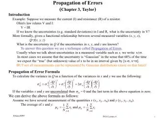
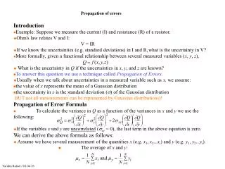
IntroductionlExample: Suppose we measure the current (I) and resistance (R) of a resistor.uOhm's law relates V and I: V = IRuIf we know the uncertainties (e.g. standard deviations) in I and R, what is the uncertainty in V?lMore formally, given a functional relationship between several measured variables (x, y, z),u What is the uncertainty in Q if the uncertainties in x, y, and z are known?nTo answer this question we use a technique called Propagation of Errors.uUsually when we talk about uncertainties in a measured variable such as x, we assume:nthe value of x represents the mean of a Gaussian distributionnthe uncertainty in x is the standard deviation () of the Gaussian distribution BUT not all measurements can be represented by Gaussian distributions)!Propagation of Error Formulal To calculate the variance in Q as a function of the variances in x and y we use the following:uIf the variables x and y are uncorrelated (xy = 0), the last term in the above equation is zero.We can derive the above formula as follows:u Assume we have several measurement of the quantities x (e.g. x1, x2...xi) and y (e.g. y1, y2...yi).n The average of x and y: Propagation of errors Yarulin Rafael / 01.04.16
udefine:evaluated at the average valuesuexpand Qi about the average values:uassume the measured values are close to the average valuesLet’s neglect the higher order terms:u If the measurements are uncorrelated the summation in the above equation is zero Since the derivatives are evaluated at the average values (mx, my) we can pull them out of the summation uncorrelated errors Yarulin Rafael / 01.04.16
If x and y are correlated, define xy as: Example: Power in an electric circuit. P = I2R Let I = 1.0 ± 0.1 amp and R = 10. ± 1.0 P = 10 watts calculate the variance in the power using propagation of errors assuming I and R are uncorrelated P = 10± 2 watts If the true value of the power was 10 W and we measured it many times with an uncertainty (s) of ± 2 W and gaussian statistics apply then 68% of the measurements would lie in the range [8,12] watts Sometimes it is convenient to put the above calculation in terms of relative errors: In this example the uncertainty in the current dominates the uncertainty in the power! Thus the current must be measured more precisely if we want to reduce the uncertainty in the power correlated errors Yarulin Rafael / 01.04.16
lExample: The error in the average (“error in the mean”). u The average of several measurements each with the same uncertainty (s) is given by:We can determine the mean better by combining measurements.But the precision only increases as the square root of the number of measurements.Do not confusesmwiths ! nsis related to the width of the Gaussian that the measurements come from. ns does not get smaller as we combine measurements.Problem in the Propagation of Errorsl In calculating the variance using propagation of errors:u We usually assume the error in measured variable (e.g. x) is Gaussian.BUT if x is described by a Gaussian distributionf(x) may not be described by a Gaussian distribution! Yarulin Rafael / 01.04.16
lWhat does the standard deviation that we calculate from propagation of errors mean?uExample: The new distribution is Gaussian.nLet y = Ax, with A = a constant and x a Gaussian variable.y= Ax and y= AxnLet the probabilitydistribution for x be Gaussian:Thus the new probability distribution for y, p(y, y, y), is also described by a Gaussian. 100 y = 2x with x = 10 ± 2 sy= 2sx= 4 80 Start with a Gaussian with m= 10, s= 2 Get another Gaussian with m= 20, s= 4 60 dN/dy 40 y 20 0 0 10 20 30 40 Yarulin Rafael / 01.04.16
100 y = 2/x with x = 10 ± 2 uExample: When the new distribution is non-Gaussian: y = 2/x.nThe transformed probability distribution function for y does not have the form of a Gaussian.l Unphysical situations can arise if we use the propagation of errors results blindly!u Example: Suppose we measure the volume of a cylinder: V = pR2L. nLet R = 1 cm exact, and L = 1.0 ± 0.5 cm.nUsing propagation of errors:sV = pR2sL = p/2 cm3.V = p ± p/2 cm3nIf the error on V (sV) is to be interpreted in the Gaussian sense then there is a finite probability (≈ 3%) that the volume (V) is < 0 since V is only 2s away from 0! Clearly this is unphysical! Care must be taken in interpreting the meaning of sV. sy= 2sx /x2 80 Start with a Gaussian with m= 10, s= 2. DO NOT get another Gaussian! 60 dN/dy 40 20 0 0.1 0.2 0.3 0.4 0.5 0.6 y Yarulin Rafael / 01.04.16