Download
1 / 35
350 likes | 479 Vues
This document provides a comprehensive overview of error analysis and propagation methods in GIS, essential for accurate spatial data interpretation. Emphasizing the significance of confidence levels in analysis, it explores various error sources, including natural variation and data collection methods. The Monte Carlo simulation technique is highlighted as a tool for assessing uncertainties in complex models. Readers will learn how to utilize Excel for generating normally distributed random samples, facilitating statistical analysis and improving data reliability.

E N D
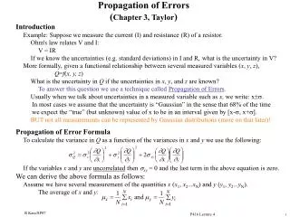
Analysis and propagation of errors Peter Fox GIS for Science ERTH 4750 (98271) Week 8, Tuesday, March 20, 2012
Contents • Error!!! • Projects • Lab assignment on Friday
Spatial analysis of continuous fields • Possibly more important than our answer is our confidence in the answer. • Our confidence is quantified by uncertainties as discussed earlier. • Once we combine numbers, we need to be able to assess how the uncertainties change for the combination. • This is called propagation of errors or more correctly the propagation of our understanding/ estimate of errors in the result we are looking at…
Types of errors • Mistakes • Natural variation • Systematic and random equipment problems • Data collection methods • Observer diligence • Locations errors/accuracy • Rasterizing and digitizing • Mismatch of data collected by different methods (e.g., seafloor bathymetry)
Reliability • Changes in data over time • Non-uniform coverage • Map scales • Observation density • Sampling theorem (aliasing) • Surrogate data and their relevance • Round-off errors in computers
Error propagation • Errors arise from data quality, model quality and data/model interaction. • We need to know the sources of the errors and how they propagate through our model. • Simplest representation of errors is to treat observations/attributes as statistical data – use mean and standard deviation.
Analytic approaches Addition and subtraction
Monte Carlo simulation • If a new attribute U is given by U = f (A1, A2, A3, …. An) where the A’s are attributes and f represents some function combining them, then we want to know what is the standard deviation of the combination U and how does the standard deviation of each A contribute to it? • By MC simulation we look at the statistical distribution of a lot of realizations (random samples) of U.
MC (ctd) • A single realization of U is Ui = f (R1, R2, R3, …. Rn) where each Rn is a random sample of its corresponding attribute An based on the statistical properties (mean and standard deviation, for example) of An. • The probability functions for the attributes themselves need not be Gaussian and could even be taken from histograms of observed values.
Recall… • The mean and standard deviation of U is estimated by • m = N-1 SUM i=1,N (Ui) • s2 = (N-1)-1 SUM i=1,N (Ui - m)2 • where N is a very large number of realizations (hundreds or thousands).
When to use? • MC simulation is most useful when the function relating the attributes is complex or the statistical distribution is known only empirically (from a histogram, for example). • For simpler combinations of attributes, there are easier, direct (analytical) ways to estimate the new uncertainties from the attribute uncertainties.
Generating pseudo random numbers • For the Monte Carlo simulation, you will want to generate a series of random numbers with a normal (bell-curve) distribution. • There are 2 ways to do this in Excel. • In older versions of Excel, you can use the Tools > Data Analysis > Random number generation > Normal distribution to generate a sequence of random numbers.
Second way • Or, you can take advantage of the central limit theorem that states that under certain conditions, random samples of any distribution will have a normal distribution. • The Excel function RAND generates a uniformly distributed random number, that is, the probability is the same for any number between 0 and 1 to be generated. • To get a normally distributed random sample with mean of 0 and standard deviation of 1 we can simply add 12 uniformly distributed random numbers and subtract 6.
To get a normally distributed random sample with mean of m and standard deviation of s we use: • [ SUM i=1,12 RAND() - 6 ] * s + m • In Matlab – RAND • In R – randu, seed, sample
Tip • Because this expression is quite long in Excel you can create a macro to facilitate using it again and again. • To record a macro, select Tools > Macro > Record new macro > give name to the macro > ok > type in expression > Stop recording. • You can refer to re-named cells from within a macro, so you might want to use variable names for the mean and standard deviation to keep your macro general.
Shortcuts • You can also specify a Control-key to run the macro from the worksheet. Otherwise, to run the macro, go to Tools > Macro > Macros > select the macro name and press Run. • Once the macro is run in a cell, you can drag the expression to other cells using the drag handle in the lower-right corner of the cell.
Statistical ‘tests’ • F-test: test if two distributions with the same mean are the same or different based on their variances and degrees of freedom. • T-test: test if two distributions with different means are the same or different based on their variances and degrees of freedom
F-test F = S12 / S22 where S1and S2 are the sample variances. The more this ratio deviates from 1, the stronger the evidence for unequal population variances.
Dealing with errors • In analyses: • report on the statistical properties • does it pass tests at some confidence level? • On maps: • exclude data that are not reliable (map only subset of data) • show additional map of some measure of confidence
Elevation map meters
Elevation errors meters
Summary • Topics for GIS (for Science) • Estimating, propagating and displaying error considerations • For learning purposes remember: • Demonstrate proficiency in using geospatial applications and tools (commercial and open-source). • Present verbally relational analysis and interpretation of a variety of spatial data on maps. • Demonstrate skill in applying database concepts to build and manipulate a spatial database, SQL, spatial queries, and integration of graphic and tabular data. • Demonstrate intermediate knowledge of geospatial analysis methods and their applications.
Friday Mar. 23 • Lab assignment session – three problems, up on ~ Wednesday • Complete them in class, get signed off before leaving • 10% of grade
Reading for this week • http://www.chemtopics.com/aplab/errors.pdf • http://www.nuim.ie/staff/dpringle/gis/gis11.pdf
Next classes • Friday, March 23 – lab with material from week 7 (lab assignment 10%) • Tuesday, March 27, Using uncertainties, working with discrete entity types • Note March 30 – open lab (no assignment, work on your projects, get help from Max), attendance will be taken