
Divide and Conquer Sorting
E N D
Presentation Transcript
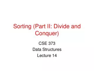
Divide and Conquer Sorting Data Structures
Insertion Sort • What if first k elements of array are already sorted? • 4, 7, 12,5, 19, 16 • We can shift the tail of the sorted elements list down and then insert next element into proper position and we get k+1 sorted elements • 4, 5, 7, 12, 19, 16
“Divide and Conquer” • Very important strategy in computer science: • Divide problem into smaller parts • Independently solve the parts • Combine these solutions to get overall solution • Idea 1: Divide array into two halves, recursively sort left and right halves, then merge two halves known as Mergesort • Idea 2 : Partition array into small items and large items, then recursively sort the two sets known as Quicksort
Mergesort • Divide it in two at the midpoint • Conquer each side in turn (by recursively sorting) • Merge two halves together 8 2 9 4 5 3 1 6
Mergesort Example 8 2 9 4 5 3 1 6 Divide 8 2 9 4 5 3 1 6 Divide 9 4 1 6 8 2 5 3 Divide 1 element 82945316 Merge 2 84 93 51 6 Merge 2 4 8 91 3 5 6 Merge 1 2 3 4 5 6 8 9
Auxiliary Array • The merging requires an auxiliary array. 2 4 8 9 1 3 5 6 Auxiliary array
Auxiliary Array • The merging requires an auxiliary array. 2 4 8 9 1 3 5 6 Auxiliary array 1
Auxiliary Array • The merging requires an auxiliary array. 2 4 8 9 1 3 5 6 Auxiliary array 1 2 3 4 5
Merging j i normal target Left completed first i j copy target
Merging first j i Right completed first second target
Merging Merge(A[], T[] : integer array, left, right : integer) : { mid, i, j, k, l, target : integer; mid := (right + left)/2; i := left; j := mid + 1; target := left; while i < mid and j < right do if A[i] < A[j] then T[target] := A[i] ; i:= i + 1; else T[target] := A[j]; j := j + 1; target := target + 1; if i > mid then //left completed// for k := left to target-1 do A[k] := T[k]; if j > right then //right completed// k : = mid; l := right; while k > i do A[l] := A[k]; k := k-1; l := l-1; for k := left to target-1 do A[k] := T[k]; }
Recursive Mergesort Mergesort(A[], T[] : integer array, left, right : integer) : { if left < right then mid := (left + right)/2; Mergesort(A,T,left,mid); Mergesort(A,T,mid+1,right); Merge(A,T,left,right); } MainMergesort(A[1..n]: integer array, n : integer) : { T[1..n]: integer array; Mergesort[A,T,1,n]; }
Iterative Mergesort Merge by 1 Merge by 2 Merge by 4 Merge by 8
Iterative Mergesort Merge by 1 Merge by 2 Merge by 4 Merge by 8 Merge by 16 copy
Iterative pseudocode • Sort(array A of length N) • Let m = 2, let B be temp array of length N • While m<N • For i = 1…N in increments of m • merge A[i…i+m/2] and A[i+m/2…i+m] into B[i…i+m] • Swap role of A and B • m=m*2 • If needed, copy B back to A
Mergesort Analysis • Let T(N) be the running time for an array of N elements • Mergesort divides array in half and calls itself on the two halves. After returning, it merges both halves using a temporary array • Each recursive call takes T(N/2) and merging takes O(N)
Mergesort Recurrence Relation • The recurrence relation for T(N) is: • T(1) < c • base case: 1 element array constant time • T(N) < 2T(N/2) + dN • Sorting n elements takes • the time to sort the left half • plus the time to sort the right half • plus an O(N) time to merge the two halves • T(N) = O(N log N)
Properties of Mergesort • Not in-place • Requires an auxiliary array • Very few comparisons • Iterative Mergesort reduces copying.
Quicksort • Quicksort uses a divide and conquer strategy, but does not require the O(N) extra space that MergeSort does • Partition array into left and right sub-arrays • the elements in left sub-array are all less than pivot • elements in right sub-array are all greater than pivot • Recursively sort left and right sub-arrays • Concatenate left and right sub-arrays in O(1) time
“Four easy steps” • To sort an array S • If the number of elements in S is 0 or 1, then return. The array is sorted. • Pick an element v in S. This is the pivot value. • Partition S-{v} into two disjoint subsets, S1 = {all values xv}, and S2 = {all values xv}. • Return QuickSort(S1), v, QuickSort(S2)
The steps of QuickSort S select pivot value 81 31 57 43 13 75 92 0 26 65 S1 S2 partition S 0 31 75 43 65 13 81 92 26 57 QuickSort(S1) and QuickSort(S2) S1 S2 0 13 26 31 43 57 75 81 92 65 S Presto! S is sorted 0 13 26 31 43 57 65 75 81 92 [Weiss]
Details, details • “The algorithm so far lacks quite a few of the details” • Picking the pivot • want a value that will cause |S1| and |S2| to be non-zero, and close to equal in size if possible • Implementing the actual partitioning • Dealing with cases where the element equals the pivot
Alternative Pivot Rules • Chose A[left] • Fast, but too biased, enables worst-case • Chose A[random], left < random < right • Completely unbiased • Will cause relatively even split, but slow • Median of three, A[left], A[right], A[(left+right)/2] • The standard, tends to be unbiased, and does a little sorting on the side.
Quicksort Partitioning • Need to partition the array into left and right sub-arrays • the elements in left sub-array are pivot • elements in right sub-array are pivot • How do the elements get to the correct partition? • Choose an element from the array as the pivot • Make one pass through the rest of the array and swap as needed to put elements in partitions
Example 0 1 2 3 4 5 6 7 8 9 8 1 4 9 0 3 5 2 7 6 0 1 4 9 7 3 5 2 6 8 i j Choose the pivot as the median of three. Place the pivot and the largest at the rightand the smallest at the left
Partitioning is done In-Place • One implementation (there are others) • median3 finds pivot and sorts left, center, right • Swap pivot with next to last element • Set pointers i and j to start and end of array • Increment i until you hit element A[i] > pivot • Decrement j until you hit element A[j] < pivot • Swap A[i] and A[j] • Repeat until i and j cross • Swap pivot (= A[N-2]) with A[i]
Example i j 0 1 4 9 7 3 5 2 6 8 i j 0 1 4 9 7 3 5 2 6 8 i j 0 1 4 9 7 3 5 2 6 8 i j 0 1 4 2 7 3 5 9 6 8 Move i to the right to be larger than pivot. Move j to the left to be smaller than pivot. Swap
Example i j 0 1 4 2 7 3 5 9 6 8 i j 0 1 4 2 7 3 5 9 6 8 i j 0 1 4 2 5 3 7 9 6 8 i j 0 1 4 2 5 3 7 9 6 8 j i 0 1 4 2 5 3 7 9 6 8 j i 0 1 4 2 5 3 6 9 7 8 pivot S1 < pivot S2 > pivot
Recursive Quicksort Quicksort(A[]: integer array, left,right : integer): { pivotindex : integer; if left + CUTOFF right then pivot := median3(A,left,right); pivotindex := Partition(A,left,right-1,pivot); Quicksort(A, left, pivotindex – 1); Quicksort(A, pivotindex + 1, right); else Insertionsort(A,left,right); } Don’t use quicksort for small arrays. CUTOFF = 10 is reasonable.
Quicksort Best Case Performance • Algorithm always chooses best pivot and splits sub-arrays in half at each recursion • T(0) = T(1) = O(1) • constant time if 0 or 1 element • For N > 1, 2 recursive calls plus linear time for partitioning • T(N) = 2T(N/2) + O(N) • Same recurrence relation as Mergesort • T(N) = O(N log N)
Quicksort Worst Case Performance • Algorithm always chooses the worst pivot – one sub-array is empty at each recursion • T(N) a for N C • T(N) T(N-1) + bN • T(N-2) + b(N-1) + bN • T(C) + b(C+1)+ … + bN • a +b(C + C+1 + C+2 + … + N) • T(N) = O(N2) • Fortunately, average case performance is O(N log N) (see text for proof)
Properties of Quicksort • No iterative version (without using a stack). • Pure quicksort not good for small arrays. • “In-place”, but uses auxiliary storage because of recursive calls. • O(n log n) average case performance, but O(n2) worst case performance.
Folklore • “Quicksort is the best in-memory sorting algorithm.” • Mergesort and Quicksort make different tradeoffs regarding the cost of comparison and the cost of a swap
Features of Sorting Algorithms • In-place • Sorted items occupy the same space as the original items. (No copying required, only O(1) extra space if any.) • Stable • Items in input with the same value end up in the same order as when they began.
How fast can we sort? • Heapsort, Mergesort, and Quicksort all run in O(N log N) best case running time • Can we do any better? • No, if the basic action is a comparison.
Sorting Model • Recall our basic assumption: we can only compare two elements at a time • we can only reduce the possible solution space by half each time we make a comparison • Suppose you are given N elements • Assume no duplicates • How many possible orderings can you get? • Example: a, b, c (N = 3)
Permutations • How many possible orderings can you get? • Example: a, b, c (N = 3) • (a b c), (a c b), (b a c), (b c a), (c a b), (c b a) • 6 orderings = 3•2•1 = 3! (ie, “3 factorial”) • All the possible permutations of a set of 3 elements • For N elements • N choices for the first position, (N-1) choices for the second position, …, (2) choices, 1 choice • N(N-1)(N-2)(2)(1)= N! possible orderings
Decision Tree a < b < c, b < c < a, c < a < b, a < c < b, b < a < c, c < b < a a > b a < b a < b < c c < a < b a < c < b b < c < a b < a < c c < b < a b < c b > c a < c a > c b < c < a b < a < c c < b < a a < b < c a < c < b c < a < b c < a c > a b < c b > c b < c < a b < a < c a < c < b a < b < c The leaves contain all the possible orderings of a, b, c
Decision Trees • A Decision Tree is a Binary Tree such that: • Each node = a set of orderings • ie, the remaining solution space • Each edge = 1 comparison • Each leaf = 1 unique ordering • How many leaves for N distinct elements? • N!, ie, a leaf for each possible ordering • Only 1 leaf has the ordering that is the desired correctly sorted arrangement
Decision Tree Example a < b < c, b < c < a, c < a < b, a < c < b, b < a < c, c < b < a possible orders a > b a < b a < b < c c < a < b a < c < b b < c < a b < a < c c < b < a b < c b > c a < c a > c b < c < a b < a < c c < b < a a < b < c a < c < b c < a < b c < a c > a b < c b > c actual order b < c < a b < a < c a < c < b a < b < c
Decision Trees and Sorting • Every sorting algorithm corresponds to a decision tree • Finds correct leaf by choosing edges to follow • ie, by making comparisons • Each decision reduces the possible solution space by one half • Run time is maximum no. of comparisons • maximum number of comparisons is the length of the longest path in the decision tree, i.e. the height of the tree
Lower bound on Height • A binary tree of height h has at mosthow many leaves? • The decision tree has how many leaves: • A binary tree with L leaves has height at least: • So the decision tree has height:
log(N!) is (NlogN) select just the first N/2 terms each of the selected terms is logN/2
(N log N) • Run time of any comparison-based sorting algorithm is (N log N) • Can we do better if we don’t use comparisons?
BucketSort (aka BinSort) If all values to be sorted are known to be between 1 andK, create an array count of size K, increment counts while traversing the input, and finally output the result. ExampleK=5. Input = (5,1,3,4,3,2,1,1,5,4,5) Running time to sort n items?
BucketSort Complexity: O(n+K) • Case 1: K is a constant • BinSort is linear time • Case 2: K is variable • Not simply linear time • Case 3: K is constant but large (e.g. 232) • ??? Impractical! Linear time sounds great. How to fix???
Fixing impracticality: RadixSort • Radix = “The base of a number system” • We’ll use 10 for convenience, but could be anything • Idea: BucketSort on each digit, least significant to most significant (lsd to msd)
Radix Sort Example (1st pass) Bucket sort by 1’s digit After 1st pass Input data 721 3 123 537 67 478 38 9 478 537 9 0 1 2 3 4 5 6 7 8 9 721 721 3 123 537 67 478 38 9 3 38 123 67 This example uses B=10 and base 10 digits for simplicity of demonstration. Larger bucket counts should be used in an actual implementation.
Radix Sort Example (2nd pass) Bucket sort by 10’s digit After 1st pass After 2nd pass 3 9 721 123 537 38 67 478 721 3 123 537 67 478 38 9 0 1 2 3 4 5 6 7 8 9 03 09 721 123 537 38 67 478
Radix Sort Example (3rd pass) Bucket sort by 100’s digit After 2nd pass After 3rd pass 3 9 721 123 537 38 67 478 3 9 38 67 123 478 537 721 0 1 2 3 4 5 6 7 8 9 003 009 038 067 123 478 537 721 Invariant: after k passes the low order k digits are sorted.