
Z L
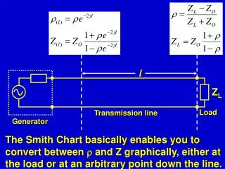
l. Z L. Load. Transmission line. Generator. The Smith Chart basically enables you to convert between and Z graphically, either at the load or at an arbitrary point down the line. Z L.

Z L
E N D
Presentation Transcript
l ZL Load Transmission line Generator The Smith Chart basically enables you to convert between and Z graphically, either at the load or at an arbitrary point down the line.
ZL To avoid having to use a different Smith Chart for every value of Zo, the normalised impedance, z , is used: z = ZL/ Zo The normalised impedance z can then be “denormalised” to obtain the load impedance ZL by multiplying by Zo: ZL = z.Zo In terms of its real and imaginary components, the normalised impedance can be written as: z = r + jx
MAPPING BETWEEN IMPEDANCE PLANE AND THE SMITH CHART r is the normalised resistance axis x is the normalised reactance axis Lines of constant normalised resistance Lines of constant normalised reactance r = 0 1 0.5 2 0.4 0.2 0 -0.2 -0.4 x = X/Zo 3 0.2 5 x = 0 10 x r = R/Zo 0 0.2 0.5 1 2 3 5 10 r 0.2 0.4 0.6 0.8 0 -10 -5 -0.2 -3 -2 -0.5 Complex (Normalised) Impedance Plane -1 Smith Chart
Pure Reactance 1 Pure Resistance 0.5 2 3 0.2 5 Matched Load 10 x 0 0.2 0.5 1 2 3 5 10 0 r -10 Short Circuit Open Circuit -5 -0.2 -3 -2 -0.5 -1
l ZL Load Transmission line Generator 1 0.5 2 3 z = r+jx of ZL only 0.2 5 || 10 x 2βl 10 0 0.2 0.5 1 2 3 5 10 2βl r 0 -10 -5 of ZL plus line of length l -0.2 z of load and line of length l -3 -2 -0.5 Point rotates clockwise by 2βl radians (2x360 l/λ degrees) at a constant radius -1 Reflection Coefficient Plane Smith Chart
l ZL “Clockwise towards generator” Load Transmission line Generator 1 0.5 2 3 z = r+jx of ZL only 0.2 5 || 10 x 2βl 10 0 0.2 0.5 1 2 3 5 10 2βl r 0 -10 -5 of ZL plus line of length l -0.2 z of load and line of length l -3 -2 -0.5 -1 Point rotates clockwise by 2βl radians (2x360 l/λ degrees) Reflection Coefficient Plane Smith Chart
Part 3 - The Smith Chart and its Applications Lec. 9 Smith Chart and General Transmission Lines Smith Chart and Variation of Frequency Smith Chart and VSWR Adding Components Using a Smith Chart Smith Chart and Matching with Series Components Admittance Using a Smith Chart Single Stub Matching
THE SMITH CHART AND VSWR for a lossless line Dividing by Zo to get the normalised impedance: r= |r|ej where θ = - 2l But - 2l is the phase difference between V+ and V-
Total voltage and impedance are a maximum when θ= - 2l = 0 or integer x 2o Voltage amplitude |V| l/4 Vmax Vmin Current amplitude | I | x x = 0 l/4 Imax Imin Impedance magnitude |Z| |Z|=|V| / | I | x x = 0 l/4 Zmax Zmin x x = 0
So, if θ = - 2βl = 0 then the magnitude of the impedance of the load and line at that point (and hence the magnitude of the normalised impedance) will be a maximum:
1 0.5 2 |r| circle zL r 3 0.2 5 10 x 10 0 0.2 0.5 1 2 3 5 10 r 0 r= |r|ej0 -10 -5 -0.2 -3 -2 -0.5 -1 Reflection Coefficient Plane Smith Chart Imaginary r |r| r-l 2l θ = - 2l Real VSWR ≡ zmax
ADDING COMPONENTS USING A SMITH CHART +j0.7 0.5 Final load +j1.0 New total impedance is 0.5 + j1.0 1 1 0.5 0.5 2 2 3 3 0.2 0.2 5 5 zL +j0.7 10 10 x x 0 0.2 0.5 1 2 3 5 10 0 0.2 0.5 1 2 3 5 10 r r 0 0 -10 -10 -5 -5 -0.2 -0.2 -3 -3 -2 -2 -0.5 -0.5 -1 -1 0.5 +j0.3 Initial load 0.3 z’L
1 0.5 2 3 0.2 5 10 x 0 0.2 0.5 1 2 3 5 10 0 r -10 -5 -0.2 -3 -2 -0.5 -1 r = 0.5 Series L x = j0.3 Series R Series C
MATCHING USING THE SMITH CHART AND SERIES COMPONENTS ZL= Zo – Load and line are matched -j25 Ω Zo = 50Ω j25 Ω j25 Ω 50 Ω 50 Ω 50 Ω 1 Add series capacitor with Xc = 1/jωC = -j25 Ω 0.5 2 3 zL 0.2 5 zL = ZL/Zo = (50+j25)/50 = 1 + j0.5 z’L = ZL/Zo = (50+j25-j25)/50 = 1 + j0 10 x 0 0.2 0.5 1 2 3 5 10 r 0 z’L -10 -5 -0.2 -3 -2 -0.5 -1
1 0.5 2 3 0.2 5 10 x 0 0.2 0.5 1 2 3 5 10 0 r -10 -5 -0.2 -3 -2 -0.5 -1 r = 0.5 Series L x = j0.3 Series R Series C
ADDING COMPONENTS IN PARALLEL WITH ZL X -j25 Ω Z Zm ZL but: 1 1 1 Z Zm ZL = + Y Ym YL Y = Ym + YL ADMITTANCES Zo = 50Ω j25 Ω 50 Ω Z Zm + ZL = = =
ADMITTANCE USING A SMITH CHART So far we have used the Smith Chart to convert between Z and or vice-versa. However, a given load has a unique value of irrespective of whether the load is expressed as an admittance or an impedance. def Y = 1/Z Minus sign means that the ADMITTANCE SMITH CHART has the same form as the impedance Smith Chart but is rotated by 180º.
1 0.5 2 3 0.2 5 10 0 0.2 0.5 1 2 3 5 10 0 -10 -5 -0.2 -3 -2 -0.5 -1 ZL = R + jX zL = r + jx 1/ZL = YL = G + jB yL = YL/Yo = g + jb -1 -0.5 -2 -3 -0.2 -5 -10 x 10 5 3 2 1 0.5 0.2 0 r g 0 b 10 5 0.2 3 2 0.5 1 ADMITTANCE SMITH CHART IMPEDANCE SMITH CHART g – normalised conductance b – normalised susceptance
ZL = R + jX (inductor or capacitor in series with R) YL = G + jB (inductor or capacitor in parallel with R) R G=1/R’ jB = 1/jX’ YL: ZL: jX jX’ R’ YL = 1/ZL = 1/R’ + 1/jX’ [R’R, X’X] Note that ZL and YL correspond to the same load and so have the same reflection coefficient.
-1 -0.5 -2 -3 -5 -10 b g 10 5 0.2 3 2 0.5 1 REFLECTION COEFFICIENT CIRCLE || ADMITTANCE SMITH CHART IMPEDANCE SMITH CHART ZL = R + jX zL = r + jx 1/ZL = YL = G + jB yL = YL/Yo = g + jb 1 0.5 2 3 -0.2 0.2 5 10 x 10 5 3 2 1 0.5 0.2 0 0 0.2 0.5 1 2 3 5 10 r 0 0 -10 -5 -0.2 -3 -2 -0.5 -1
1 0.5 2 3 0.2 5 10 0 0.2 0.5 1 2 3 5 10 0 -10 -5 -0.2 b g -3 -2 -0.5 -1 ADMITTANCE SMITH CHART IMPEDANCE SMITH CHART x r
R 1 0.5 2 3 0.2 5 10 0 0.2 0.5 1 2 3 5 10 0 -10 -5 -0.2 -3 -2 -0.5 -1 IMPEDANCE SMITH CHART ZL = R + jX zL = r + jx jX x r YL = G + jB yL = g + jb jB G G=1/R’ ; jB = 1/jX’
SINGLE STUB MATCHING In general, the load will not match the values of Zo available – a fraction ||2 of the power will bounce back up the line Forward power Backward power ZL Zo Load Transmission line (Zo) Source To overcome this problem we need to add a circuit in front of the load which makes it look like an impedance Zo. Z = Zo Matching circuit or network ZL Zo Forward power only Load Transmission line (Zo) Source
A transmission line terminated in a short circuit or an open circuit has an impedance that is purely reactive – i.e. it looks like a capacitor or an inductor For a lossless line: For a short circuit termination ZL = 0, hence:
For a lossless line: For an open circuit termination ZL = , hence: By adjusting the length, l, of the line from 0 to λ/2 the reactance of the line can be made to have any value from − to + i.e. all possible values of capacitance and inductance.
SINGLE STUB MATCHING Either short-circuit or open-circuit ls the “stub” Zo ZL Zo ys Load Zo lm ym Transmission line (Zo) Source Adjust lm until ym = 1 + jb Adjust ls until ys = - jb Total admittance y = ym + ys = 1 y = 1 YL’/Yo (= Zo/ZL’) = 1 – line now matched (ZL’ is the impedance of load + added section + stub)
ys (a) Plot zL 1 (d) Rotate clockwise to y = 1 + jb circle – angle (2lm) gives lm 1+jb circle (b) Draw circle through zL 0.5 2 3 (c) Go 180º round chart to yL (e) Read off normalised susceptance, b, for ym 0.2 5 yL open circuit 10 b 0 0.2 0.5 1 2 3 5 10 0 g (f) Plot negative of b on chart – this is ys , target susceptance for the stub. -10 zL -5 -0.2 ym -3 (g) Rotate clockwise from y=0 (open circuit) or y= (short circuit) to ys – angle (2ls) gives ls short circuit -2 -0.5 b for ym -1
SINGLE STUB MATCHING Either short-circuit or open-circuit ls the “stub” Zo ZL Zo ys Load Zo lm ym Transmission line (Zo) Source Adjust lm until ym = 1 + jb Adjust ls until ys = - jb Total admittance y = ym + ys = 1 y = 1 YL’/Yo (= Zo/ZL’) = 1 – line now matched (ZL’ is the impedance of load + added section + stub)
Tutorial D, Question 6 A transmitter and transmission line with Zo = 300 Ω are to feed a 75 Ω aerial. The frequency of operation is 400 MHz and the phase velocity on the line is 3 x 10⁸ m/s. Design a single-stub matching network, using an open-circuited stub.
Tutorial D, Question 6 λ = v/f = 3x10⁸/4x108 = 0.75m • Plot zL on Smith Chart: • zL = ZL/Zo • = 75/300 • = 0.25+j0 1+jb circle yL zL 2. Rotate 180º around chart to yL 53º ym 3. Rotate clockwise to 1+jb circle lm= 53ºxλ/(2x360°) = 55.2mm
4. Read off susceptance of ym : -j1.52 ys=+j1.52 5. Plot –ve of ym susceptance on chart: ys = +j1.52 113º zL yL 53º y=0 6. Open circuit termination, so start at y=0, rotate clockwise to ys : ls= 113ºxλ/(2x360°) = 118mm ym
THE SMITH CHART AND VSWR • The normalised impedance of a load and line combination is a maximum, zmax, when - 2l = θ = 0 • zmax = VSWR zL • Intersection of circle through load point, zL, with right-hand half of resistance axis gives VSWR and zmax.
Adding components in series with load: Adding inductors: move clockwise around constant r circle Adding capacitors: move anticlockwise around constant r circle Adding resistors: move along arc of constant x towards r-axis
ADMITTANCE SMITH CHART is identical with the impedance Smith Chart but rotated by 180º. • central axis is normalised conductance • outer axis is normalised susceptance • Admittance Smith Chart can be used for adding components in parallel with the load and converting between impedance and admittance.
Matching involves inserting between the load and the end of the line a “circuit” such that the combined impedance of the load and “circuit” is Zo. Z = Zo Matching circuit or network ZL Zo Forward power only Load Transmission line (Zo) Source
ZL Zo Load Zo lm SINGLE STUB MATCHING • In SINGLE STUB MATCHING the “circuit” consists of 2 sections of transmission line, one connected between the load and the end of the line, and a second (the “stub”) connected in parallel. Either short-circuit or open-circuit ls the “stub” Zo ys ym Transmission line (Zo)
ZL Zo Load Zo lm • A section of transmission line terminated in an open-circuit or short-circuit has a pure reactance – it can be given any reactance value between + and − simply by adjusting its length. For short-circuit: Either short-circuit or open-circuit For open-circuit: ls the “stub” Zo ys ym