Chapter 8 IIR Filter Design

1. Chapter 8 IIR Filter Design Gao Xinbo School of E.E., Xidian Univ. Xbgao@ieee.org http://see.xidian.edu.cn/teach/matlabdsp/

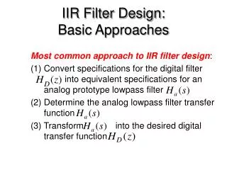
2. Introduction • IIR filter have infinite-duration impulse responses, hence they can be matched to analog filters, all of which generally have infinitely long impulse responses. • The basic technique of IIR filter design transforms well-known analog filters into digital filters using complex-valued mappings. • The advantage of this technique lies in the fact that both analog filter design (AFD) tables and the mappings are available extensively in the literature.

3. Introduction • The basic technique is called the A/D filter transformation. • However, the AFD tables are available only for lowpass filters. We also want design other frequency-selective filters (highpass, bandpass, bandstop, etc.) • To do this, we need to apply frequency-band transformations to lowpass filters. These transformations are also complex-valued mappings, and they are also available in the literature.

4. Two approaches Approach 1, used in Matlab Approach 2, study

5. IIR Filter Design Steps • Design analog lowpass filter • Study and apply filter transformations to obtain digital lowpass filter • Study and apply frequency-band transformations to obtain other digital filters from digital lowpass filter

6. The main problem • We have no control over the phase characteristics of the IIR filter. • Hence IIR filter designs will be treated as magnitude-only designs.

7. Main Content of This Chapter • Analog filter specifications and the properties of the magnitude-squared response used in specifying analog filters. • Characteristics of three widely used analog filters • Butterworth, Chebyshev, and Elliptic filter • Transformation to convert these prototype analog filters into different frequency-selective digital filter

8. Some Preliminaries • Relative linear scale • The lowpass filter specifications on the magnitude-squared response are given by Where epsilon is a passband ripple parameter, Omega_p is the passband cutoff frequency in rad/sec, A is a stopband attenuation parameter, and Omega_s is the stopband cutoff in rad/sec.

10. The relations among epsilon, A, Rp, As, delta1 and delta2

11. Properties of |Ha(jOmega)|2 Analog filter specifications, which are given in terms of the magnitude-squared response, contain no phase information. Now to evaluate the s-domain system function Ha(s), consider Therefore the poles and zeros of the magnitude-squared function are distributed in a mirror-image symmetry with respect to the jOmega axis. Also for real filters, poles and zeros occur in complex conjugate pairs (or mirror-image symmetry with respect to the real axis). From this pattern we can construct Ha(s), which is the system function of our analog filter.

12. Properties of |Ha(jOmega)|2 • We want Ha(s) to represents a causal and stable filter. Then all poles of Ha(s) must lie within the left half-plane. Thus we assign all left-half poles of Ha(s)Ha(-s) to Ha(s). • We will choose the zeros of Ha(s)Ha(-s) lying inside or on the jOmega axis as the zeros of Ha(s). • The resulting filter is then called a minimum-phase filter.

13. Characteristics of Prototype Analog Filters • IIR filter design techniques rely on existing analog filter filters to obtain digital filters. We designate these analog filters as prototype filters. • Three prototypes are widely used in practice • Butterworth lowpass • Chebyshev lowpass (Type I and II) • Elliptic lowpass

14. Butterworth Lowpass Filter • This filter is characterized by the property that its magnitude response is flat in both passband and stopband. The magnitude-squared response of an N-order lowpass filter Omega_c is the cutoff frequency in rad/sec. Plot of the magnitude-squared response is shown in P.305

16. Properties of Butterworth Filter • Magnitude Response • |Ha(0)|2 =1, |Ha(jΩc) |2 =0.5, for all N (3dB attenuation at Ωc) • |Ha(jΩ)|2 monotonically decrease for Ω • Approaches to ideal filter when N→∞ To determine the system function Ha(s)

17. Poles of |Ha(jΩ)|2 Ω=s/j =Ha(s) Ha(-s) • Equally distributed on a circle of radius Ωc with angular spacing of pi/N radians • For N odd, pk= Ωcej2pik/N • For N even, pk= Ωcej(pi/2N+kpi/N) • Symmetry respect to the imaginary axis • A pole never falls on the imaginary axis, and falls on the real axis only if N is odd • A stable and causal filter Ha(s) can now be specified by selecting poles in the left half-plane Example 8.1

18. Matlab Implementation • Function [z,p,k] = buttap(N) • To design a normalized (Ωc=1) Butterworth analog prototype filter of order N • Z: zeros; p: poles; k: gain value • Function [b,a] = u_buttap(N,Omegac) • Provide a direct form (or numerator-denominator) structure. • Function [C,B,A] = sdir2cas(b,a) • Convert the direct form into the cascade form Example 8.2

19. Design Equations The analog lowpass filter is specified by the parameters, Omega_p. R_p,Omega_s, and A_s. Therefore the essence of the design in the case of Butterworth filter is to obtain the order N and the cutoff frequency Omega_c.

20. Matlab Implementation • Function [b,a] = afd_butt(Wp,Ws,Rp,As) • To design an analog Butterworth lowpass filter, given its specifications. • Function [db,mag,pha,w] = freqs_m(b,a,wmax) • Magnitude response in absolute as well as in relative dB scale and the phase response. Example 8.3

21. Chebyshev Lowpass Filter • Chebyshev-I filters • Have equiripple response in the passband • Chebyshev-II filters • Have equiripple response in stopband • Butterworth filters • Have monotonic response in both bands • We note that by choosing a filter that has an equripple rather than a monotonic behavior, we can obtain a low-order filter. • Therefore Chebyshev filters provide lower order than Buttworth filters for the same specifications.

22. The magnitude-squared response of Chebyshev-I filter N is the order of the filter, Epsilon is the passband ripple factor Nth-order Chebyshev polynomial • For 0<x<1, TN(x) oscillates between –1 and 1, and • For 1<x<infinity, TN(x) increases monotonically to infinity • Figure on P.314 (two possible shapes) • Observations: P.315

23. Observations At x=0 (or Ω=0); |Ha(j0)|2 = 1; for N odd; = 1/(1+epson^2); for N even At x=1 (or Ω= Ωc); |Ha(j1)|2= 1/(1+epson^2) for all N. For 0<=x<=1 (or 0<= Ω<= Ωc) |Ha(jx)|2 oscillates between 1 and1/(1+epson^2) For x>1 (or Ω > Ωc), |Ha(jx)|2 decreases monotonically to 0 . At x= Ωr, |Ha(jx)|2 = 1/(A^2).

24. Causal and stable Ha(s) To determine a causal and stable Ha(s), we must find the poles of Ha(s)Ha(-s) and select the left half-plane poles for Ha(s). The poles of Ha(s)Ha(-s) are obtained by finding the roots of It can be shown that if are the (left half-plane) roots of the above polynomial, then

26. The poles of Ha(s)Ha(-s) The poles fall on an ellipse with major axis b Ωc and minor axis a Ωc . Now the system function is Left half-plane K is a normalizing factor

27. Matlab Implementation • Function [z,p,k] = cheb1ap(N,Rp) • To design a normalized Chebyshev-I analog prototype filter of order N and passband ripple Rp. • Z array: zeros; poles in p array, gain value k • Function [b,a] = u_chblap(N,Rp,Omegac) • Return Ha(s) in the direct form

28. Design Equations Given Ωp, Ωs, Rp and As, three parameters are required to determine a Chebyshev-I filter Function [b,a]=afd_chb1(Wp,Ws,Rp,As) Example 8.6

29. Chebyshev-II filter Related to the Chebyshev-I filter through a simple transformation. It has a monotone passband and an equiripple stopband, which implies that this filter has both poles and zeros in the s-plane. Therefore the group delay characteristics are better (and the phase response more linear) in the passband than the Chebyshev-I prototype.

30. Matlab implementation • Function [z,p,k] = cheb2ap(N,As); • normalized Chebyshev-II • Function [b,a] = u_chb2ap(N,As,Omegac) • Unnormalized Chebyshev-II • Function [b,a] = afd_chb2(Wp,Ws,Rp,As) Example 8.7

31. Elliptic Lowpass Filters These filters exhibit equiripple behavior in the passband as well as the stopband. They are similar in magnitude response characteristics to the FIR equiripple filters. Therefore elliptic filters are optimum filters in that they achieve the minimum order N for the given specifications These filters, for obvious reasons, are very difficult to analyze and therefore, to design. It is not possible to design them using simple tools, and often programs or tables are needed to design them.

32. The magnitude-squared response N: the order; epsilon: passbang ripple; UN() is the Nth order Jacobian elliptic function Typical responses for odd and even N are shown on P.323 Computation of filter order N:

33. Matlab Implementation • [z,p,k]=ellipap(N,Rp,As); • normalized elliptic analog prototype • [b,a] = u_ellipap(N,Rp,As,Omegac) • Unnormalized elliptic analog prototype • [b,a] = afd_elip(Wp,Ws,Rp,As) • Analog Lowpass Filter Design: Elliptic • Example 8.8

34. Phase Responses of Prototype Filters • Elliptic filter provide optimal performance in the magnitude-squared response but have highly nonlinear phase response in the passband (which is undesirable in many applications). • Even though we decided not to worry about phase response in our design, phase is still an important issue in the overall system. • At other end of the performance scale are the Buttworth filters, which have maximally flat magnitude response and require a higher-order N (more poles) to achieve the same stopband specification. However, they exhibit a fairly linear phase response in their passband.

35. Phase Responses of Prototype Filters • The Chebyshev filters have phase characteristics that lie somewhere in between. • Therefore in practical applications we do consider Butterworth as well as Chebyshev filters, in addition to elliptic filters. • The choice depends on both the filter order (which influences processing speed and implementation complexity) and the phase characteristics (which control the distortion).

36. Analog-to-digital Filter Transformations • After discussing different approaches to the design of analog filters, we are now ready to transform them into digital filters. • These transformations are derived by preserving different aspects of analog and digital filters. • Impulse invariance transformation • Preserve the shape of the impulse response from A to D filter • Finite difference approximation technique • Convert a differential eq. representation into a corresponding difference eq. • Step invariance • Preserve the shape of the step response • Bilinear transformation • Preserve the system function representation from A to D domain

37. Impulse Invariance Transformation • The digital filter impulse response to look similar to that of a frequency-selective analog filter. • Sample ha(t) at some sampling interval T to obtain h(n): h(n)=ha(nT) • Since z=ejwon the unit circle and s=j Ω on the imaginary axis, we have the following transformation from the s-plane to the z-plane: z=esT Frequency-domain aliasing formula

38. Complex-plane mapping in impulse invariance transformation

39. Properties: • Sigma = Re(s): • Sigma < 0, maps into |z|<1 (inside of the UC) • Sigma = 0, maps into |z|=1 (on the UC) • Sigma >0, maps into |Z|>1 (outside of the UC) • Many s to one z mapping: many-to-one mapping • Every semi-infinite left strip (so the whole left plane) maps to inside of unit circle • Causality and Stability are the same without changing; • Aliasing occur if filter not exactly band-limited

40. Given the digital lowpass filter specifications wp,ws,Rp and As, we want to determine H(z) by first designing an equivalent analog filter and then mapping it into the desired digital filter. Design Procedure: • 1. Choose T and determine the analog frequencies: Ωp=wp/T, Ωs=ws/T • 2. Design an analog filter Ha(s) using the specifications with one of the three prototypes of the previous section. • 3. Using partial fraction expansion, expand Ha(s) into • 4. Now transform analog poles {pk} into digital poles {epkT} to obtain the digital filter Ex 8.9

41. Matlab Implementation • Function [b,a] = imp_invr(c,d,T) • b = 数字滤波器的z^(-1)分子多项式 • a = 数字滤波器的z^(-1)分母多项式 • c = 模拟滤波器的s的分子多项式 • d = 模拟滤波器的s的分母多项式 • T = 采样(变换)参数 • Examples 8.10-8.14

42. Advantages of Impulse Invariance Mapping • It is a stable design and the frequencies Ω and w are linearly related. • Disadvantage • We should expect some aliasing of the analog frequency response, and in some cases this aliasing is intolerable. • Consequently, this design method is useful only when the analog filter is essentially band-limited to a lowpass or bandpass filter in which there are no oscillations in the stopband.

43. Bilinear Transformation • This mapping is the best transformation method. Linear fractional transformation The complex plane mapping is shown in Figure 8.15

44. Complex-plane mapping in bilinear transformation

45. Observations • Sigma < 0 |z| < 1, Sigma = 0 |z| = 1, Sigma > 0 |z| > 1 • The entire left half-plane maps into the inside of the UC. This is a stable transformation. • The imaginary axis maps onto the UC in a one-to-one fashion. Hence there is no aliasing in the frequency domain. • Relation of ω to Ω is nonlinear ω= 2tan-1(ΩT/2)↔ Ω=2tan(ω/2)/T; Function [b,a] = bilinear(c,d,Fs)

46. Given the digital filter specifications wp,ws,Rp and As, we want to determine H(z). The design steps in this procedure are the following: • Choose a value for T. this is arbitrary, and we may set T = 1. • Prewarp the cutoff freq.s wp and ws; that is calculate Ωp and Ωs using (8.28) : Ωp=2/T*tan(wp/2), Ωs=2/T*tan(ws/2) • 3. Design an analog filter Ha(s) to meet the specifications. • 4. Finally set • And simplify to obtain H(z) as a rational function in z-1 Ex 8.17

47. Advantage of the bilinear Transformation • It is a stable design • There is no aliasing • There is no restriction on the type of filter that can be transformed.

48. Lowpass Design Using Matlab • Matlab Function: • [b, a] = butter(N, wn) • [b, a] = cheby1(N, Rp, wn) • [b, a] = cheby2(N, As, wn) • [b, a] = ellip(N, Rp, As, wn) • Buttord, cheb1ord, cheb2ord, ellipord can provide filter order N and filter cutoff frequency wn, given the specification.

49. Lowpass filter design • Digital filter specification • Analog prototype specifications • Analog prototype order calculation,Omega_c,wn • Digital Filter design (four types) • dir2cas

50. Digital filter design examples For the same specifications, do the following: • Ex8.21: Butterworth LP filter design; • Ex8.22: Chebyshev-I LP filter design; • Ex8.23: Chebyshev-II LP filter design; • Ex8.24: Elliptic LP filter design;