
Big Data Infrastructure
E N D
Presentation Transcript
Big Data Infrastructure CS 489/698 Big Data Infrastructure (Winter 2016) Week 5: Analyzing Graphs (1/2) February 2, 2016 Jimmy Lin David R. Cheriton School of Computer Science University of Waterloo These slides are available at http://lintool.github.io/bigdata-2016w/ This work is licensed under a Creative Commons Attribution-Noncommercial-Share Alike 3.0 United StatesSee http://creativecommons.org/licenses/by-nc-sa/3.0/us/ for details
Structure of the Course Analyzing Text Analyzing Relational Data Data Mining Analyzing Graphs “Core” framework features and algorithm design
What’s a graph? • G = (V,E), where • V represents the set of vertices (nodes) • E represents the set of edges (links) • Both vertices and edges may contain additional information • Different types of graphs: • Directed vs. undirected edges • Presence or absence of cycles • Graphs are everywhere: • Hyperlink structure of the web • Physical structure of computers on the Internet • Interstate highway system • Social networks
Some Graph Problems • Finding shortest paths • Routing Internet traffic and UPS trucks • Finding minimum spanning trees • Telco laying down fiber • Finding Max Flow • Airline scheduling • Identify “special” nodes and communities • Breaking up terrorist cells, spread of avian flu • Bipartite matching • Monster.com, Match.com • And of course... PageRank
What makes graphs hard? • Irregular structure • Irregular data access patterns • Iterations
Graphs and MapReduce (and Spark) • A large class of graph algorithms involve: • Performing computations at each node: based on node features, edge features, and local link structure • Propagating computations: “traversing” the graph • Key questions: • How do you represent graph data in MapReduce (and Spark)? • How do you traverse a graph in MapReduce (and Spark)?
Representing Graphs • G = (V, E) • Three common representations • Adjacency matrix • Adjacency list • Edge lists
Adjacency Matrices Represent a graph as an n x n square matrix M • n = |V| • Mij = 1 means a link from node i to j 2 1 3 4
Adjacency Matrices: Critique • Advantages: • Amenable to mathematical manipulation • Iteration over rows and columns corresponds to computations on outlinks and inlinks • Disadvantages: • Lots of zeros for sparse matrices • Lots of wasted space
Adjacency Lists Take adjacency matrices… and throw away all the zeros 1: 2, 4 2: 1, 3, 4 3: 1 4: 1, 3 Wait, where have we seen this before?
Adjacency Lists: Critique • Advantages: • Much more compact representation • Easy to compute over outlinks • Disadvantages: • Much more difficult to compute over inlinks
Edge Lists Explicitly enumerate all edges (1, 2) (1, 4) (2, 1) (2, 3) (2, 4) (3, 1) (4, 1) (4, 3)
Edge Lists: Critique • Why? • Edges arrive in no particular order • Sometimes, we want to store inverted edges • Advantages: • Supports the ability to perform edge partitioning • Disadvantages: • Takes a lot of space
Co-occurrence of characters in Les Misérables Source: http://bost.ocks.org/mike/miserables/
Co-occurrence of characters in Les Misérables Source: http://bost.ocks.org/mike/miserables/
Co-occurrence of characters in Les Misérables How are visualizations like this generated? Limitations? Source: http://bost.ocks.org/mike/miserables/
What does the web look like? Analysis of a large webgraph from the common crawl: 3.5 billion pages, 129 billion links Meusel et al. Graph Structure in the Web — Revisited. WWW 2014.
What does the web look like? Very roughly, a scale-free network Fraction of k nodes having k connections: (i.e., distribution follows a power law)
Power Laws are everywhere! Figure from: Newman, M. E. J. (2005) “Power laws, Pareto distributions and Zipf's law.” Contemporary Physics 46:323–351.
What does the web look like? Very roughly, a scale-free network Other Examples: Internet domain routers Co-author network Citation network Movie-Actor network Why?
(In this installment of “learn fancy terms for simple ideas”) Preferential Attachment Also: Matthew Effect For unto every one that hath shall be given, and he shall have abundance: but from him that hath not shall be taken even that which he hath. — Matthew 25:29, King James Version.
What about Facebook? Figure from: Seth A. Myers, Aneesh Sharma, Pankaj Gupta, and Jimmy Lin. Information Network or Social Network? The Structure of the Twitter Follow Graph. WWW 2014.
BTW, how do we compute these graphs? (Assume graph stored as adjacency lists)
Count. Source: http://www.flickr.com/photos/guvnah/7861418602/
BTW, how do we extract the webgraph? The webgraph… is big?! A few tricks: Integerize vertices (montone minimal perfect hashing) Sort URLs Integer compression webgraph from the common crawl: 3.5 billion pages, 129 billion links 58 GB! Meusel et al. Graph Structure in the Web — Revisited. WWW 2014.
Graphs and MapReduce (and Spark) • A large class of graph algorithms involve: • Performing computations at each node: based on node features, edge features, and local link structure • Propagating computations: “traversing” the graph • Key questions: • How do you represent graph data in MapReduce (and Spark)? • How do you traverse a graph in MapReduce (and Spark)?
Single-Source Shortest Path • Problem: find shortest path from a source node to one or more target nodes • Shortest might also mean lowest weight or cost • First, a refresher: Dijkstra’s Algorithm
Dijkstra’s Algorithm Example 1 10 0 9 2 3 4 6 7 5 2 Example from CLR
Dijkstra’s Algorithm Example 10 1 10 0 9 2 3 4 6 7 5 5 2 Example from CLR
Dijkstra’s Algorithm Example 8 14 1 10 0 9 2 3 4 6 7 5 5 7 2 Example from CLR
Dijkstra’s Algorithm Example 8 13 1 10 0 9 2 3 4 6 7 5 5 7 2 Example from CLR
Dijkstra’s Algorithm Example 8 9 1 1 10 0 9 2 3 4 6 7 5 5 7 2 Example from CLR
Dijkstra’s Algorithm Example 8 9 1 10 0 9 2 3 4 6 7 5 5 7 2 Example from CLR
Single-Source Shortest Path • Problem: find shortest path from a source node to one or more target nodes • Shortest might also mean lowest weight or cost • Single processor machine: Dijkstra’s Algorithm • MapReduce: parallel breadth-first search (BFS)
Finding the Shortest Path • Consider simple case of equal edge weights • Solution to the problem can be defined inductively • Here’s the intuition: • Define: b is reachable from a if b is on adjacency list of a DistanceTo(s) = 0 • For all nodes p reachable from s, DistanceTo(p) = 1 • For all nodes n reachable from some other set of nodes M, DistanceTo(n) = 1 + min(DistanceTo(m), mM) d1 m1 … d2 s n … m2 … d3 • m3
Visualizing Parallel BFS n7 n0 n1 n2 n3 n6 n5 n4 n8 n9
From Intuition to Algorithm • Data representation: • Key: node n • Value: d (distance from start), adjacency list (nodes reachable from n) • Initialization: for all nodes except for start node, d = • Mapper: • m adjacency list: emit (m, d + 1) • Remember to also emit distance to yourself • Sort/Shuffle • Groups distances by reachable nodes • Reducer: • Selects minimum distance path for each reachable node • Additional bookkeeping needed to keep track of actual path
Multiple Iterations Needed • Each MapReduce iteration advances the “frontier” by one hop • Subsequent iterations include more and more reachable nodes as frontier expands • Multiple iterations are needed to explore entire graph • Preserving graph structure: • Problem: Where did the adjacency list go? • Solution: mapper emits (n, adjacency list) as well Ugh! This is ugly!
Stopping Criterion • How many iterations are needed in parallel BFS (equal edge weight case)? • Convince yourself: when a node is first “discovered”, we’ve found the shortest path • Now answer the question... • Six degrees of separation? • Practicalities of implementation in MapReduce
Comparison to Dijkstra • Dijkstra’s algorithm is more efficient • At each step, only pursues edges from minimum-cost path inside frontier • MapReduce explores all paths in parallel • Lots of “waste” • Useful work is only done at the “frontier” • Why can’t we do better using MapReduce?
Single Source: Weighted Edges • Now add positive weights to the edges • Why can’t edge weights be negative? • Simple change: add weight w for each edge in adjacency list • In mapper, emit (m, d + wp) instead of (m, d + 1) for each node m • That’s it?
Stopping Criterion • How many iterations are needed in parallel BFS (positive edge weight case)? • Convince yourself: when a node is first “discovered”, we’ve found the shortest path Not true!