Simplex algorithm for problems with bounded variables
Learn how to apply the Simplex method for linear programming problems with bounded variables, including changing variable bounds to optimize solutions.

Simplex algorithm for problems with bounded variables
E N D
Presentation Transcript
Simplex algorithm for problems with bounded variables
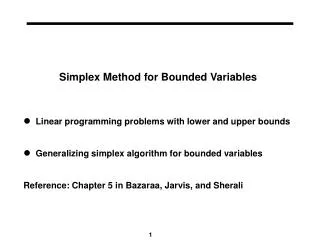
Simplex method for problems with bounded variables • Consider the linear programming problem with bounded variables • Complete the following change of variables to reduce the lower bound to 0 xj = gj – lj(i.e., gj = xj + lj)
Simplex method for problems with bounded variables the problem becomes • Complete the following change of variables to reduce the lower bound to 0 xj = gj – lj(i.e., gj = xj + lj)
Simplex method for problems with bounded variables the problem becomes replacing : uj = qj – ljand b = h – Al
Simplex method forproblems with bounded variables • In this problem since cTl is a constant, we can eliminate it from the minimisation without modifying the optimal solution. Then in the rest of the presentation we consider the problem without this constant.
Consider the explicit formulation of the problem • One way of solving the problem is to introduce slack variables yj, and then use the simplex algorithm.
Non degeneracy: all the basic variables are positive at each iteration • Consider a basic feasible solution of this problem • Because of the constraints xj+ yj = uj, at least one of the variables xjor yj is basic, j = 1,2,…,n. • Then for all j = 1,2,…,n, one of the three situations holds: a) xj= uj is basic and yj = 0 is non basic b) xj= 0 is non basic and yj = ujis basic c) 0 < xj < uj is basic and 0 < yj < uj is basic
m + n basic variables required There are n variables yj There are at least m variables xj that are basic Exactly m variables xj satisfying 0 < xj < uj. For contradiction, if m0 mvariables xj satisfy the relation, then the m0 corresponding variables yjwould be basic. Furthermore, for the n – m0 other indices j, either xj= uj(case a)or yj = uj(case b) would be verified. Then the number of basic variables would be equal to 2m0 + (n – m0) = m0 + nm + n
m + n basic variables required There are n variables yj There are at least m variables xj that are basic Exactly m variables xj satisfying 0 < xj < uj. For contradiction, if m0 mvariables xj satisfy the relation, then the m0 corresponding variables yjwould be basic. Furthermore, for the n – m0 other indices j, either xj= uj(case a)or yj = uj(case b) would be verified. Then the number of basic variables would be equal to 2m0 + (n – m0) = m0 + nm + n
La base a donc la forme suivante 0 < xj< uj 0 < yj < uj xj=uj yj=uj
The basis has the following form 0 < xj< uj 0 < yj < uj xj=uj yj=uj
The basis has the following form m Basis of A The columns of the basis B of A are those of the variables 0<xj<uj n 0 < xj< uj 0 < yj < uj xj=uj yj=uj
Then, we can specify a variant of the simplex method to solve this problem specifically: by dealing implictly with the upper bound uj. At each iteration, we consider a solution (basic) associated with a basis B de A having m basicvariables n – m non basic variables
At each iteration, we consider a solution (basic) associated with a basis B de A having m basicvariables n – m non basic variables • Denote the indices of the basic variables IB = {j1, j2, …, jm} where ji is the index of the basic variable in the ithrow, then We find similar values as in problems where there are no upper bounds, except for non basic variables
We have to modify the entering criterion and the leaving criterion accordingly to generate a variant of the simplex algorithm for this problem We find similar values as in problems where there are no upper bounds, except for non basic variables
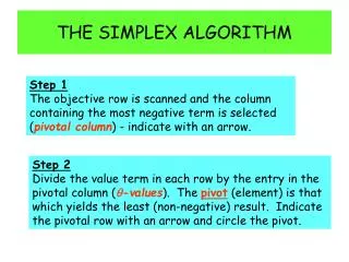
Step 1: Selecting the entering variable The criterion to select the entering variable must be modified to account for the non basic variables xjbeing equal to their upper bounds ujsince these variables can be reduced. Hence, for an index if , it is interesting to increase xj if , it is interesting to decrease xj
The increase θ of the entering variable xsis stop by the first of the following three situations happening: i) xsreach its upper bound us ii) a basic variable decreases to 0 (in this case ) iii) a basic variable increases to reach its upper bound (in ths case ) Let Step 2.1: Selecting the leaving variable Value of the basic variables
The increase θ of the entering variable xsis stop by the first of the following three situations happening: i) xsreach its upper bound us ii) a basic variable decreases to 0 (in this case ) iii) a basic variable increases to reach its upper bound (in ths case ) Let Step 2.1: Selecting the leaving variable Value of the basic variables Si θ = ∞, alors le problème n’est pas borné inférieurement et l’algorithme s’arrête.
The increase θ of the entering variable xsis stop by the first of the following three situations happening: i) xsreach its upper bound us ii) a basic variable decreases to 0 (in this case ) iii) a basic variable increases to reach its upper bound (in ths case ) Let Step 2.1: Selecting the leaving variable Value of the basic variables If θ = ∞, then the problem is not bounded from below, and the algorithm stops.
The increase θ of the entering variable xsis stop by the first of the following three situations happening: i) xsreach its upper bound us ii) a basic variable decreases to 0 (in this case ) iii) a basic variable increases to reach its upper bound (in ths case ) Let Step 2.1: Selecting the leaving variable Value of the basic variables
The increase θ of the entering variable xsis stop by the first of the following three situations happening: i) xsreach its upper bound us ii) a basic variable decreases to 0 (in this case ) iii) a basic variable increases to reach its upper bound (in ths case ) Let Step 2.1: Selecting the leaving variable Value of the basic variables
The increase θ of the entering variable xsis stop by the first of the following three situations happening: i) xsreach its upper bound us ii) a basic variable decreases to 0 (in this case ) iii) a basic variable increases to reach its upper bound (in ths case ) Let Step 2.1: Selecting the leaving variable Value of the basic variables
Step 1: Selecting the entering variable The criterion to select the entering variable must be modified to account for the non basic variables xjbeing equal to their upper bounds ujsince these variables can be reduced. Hence, for an index if , it is interesting to increase xj if , it is interesting to decrease xj
The decrease θ of the entering variable xsis stop by the first of the following three situations happening: i) xsreduces to 0 ii) a basic variable decreases to 0 (in this case ) iii) a basic variable increases to reach its upper bound (in this case ) Let Step 2.2: Selecting the leaving variable Value of the basic variables
The decrease θ of the entering variable xsis stop by the first of the following three situations happening: i) xsreduces to 0 ii) a basic variable decreases to 0 (in this case ) iii) a basic variable increases to reach its upper bound (in ths case ) Let Step 2.2: Selecting the leaving variable Value of the basic variables
The decrease θ of the entering variable xsis stop by the first of the following three situations happening: i) xsreduces to 0 ii) a basic variable decreases to 0 (in this case ) iii) a basic variable increases to reach its upper bound (in ths case ) Let Step 2.2: Selecting the leaving variable Value of the basic variables
The decrease θ of the entering variable xsis stop by the first of the following three situations happening: i) xsreduces to 0 ii) a basic variable decreases to 0 (in this case ) iii) a basic variable increases to reach its upper bound (in ths case ) Let Step 2.2: Selecting the leaving variable Value of the basic variables
The decrease θ of the entering variable xsis stop by the first of the following three situations happening: i) xsreduces to 0 ii) a basic variable decreases to 0 (in this case ) iii) a basic variable increases to reach its upper bound (in ths case ) Let Step 2.2: Selecting the leaving variable Value of the basic variables
References M.S. Bazaraa, J.J. Jarvis, H.D. Sherali, “ Linear Programming and Network Flows”, 3rd edition, Wiley-Interscience (2005), p. 217 F.S. Hillier, G.J. Lieberman, “Introduction to Operations Research”, Mc Graw Hill (2005), Section 7.3 D. G. Luenberger, “ Linear and Nonlinear Programming ”, 2nd edition, Addison-Wesley (1984), Section 3.6